Chapter 1
The question
Think of a metal part that is cooled by liquid oxygen, which boils at 90 K, and later runs at 1000 K, and then goes back again. It does this hundreds of times. If anything inside the metal changes on the way (how its atoms are arranged, how much room they take up), that change happens again on every trip. A change repeated that often builds up stress, and stress repeated that often cracks things.
This project looks for an alloy in which nothing of that kind happens between those two temperatures.
One phase, from 90 K to 1000 K
A material can hold its atoms in more than one arrangement. Ice and liquid water are the same molecules arranged two ways. In a solid metal the alternatives are subtler: the atoms may keep the same crystal but sort themselves differently, or move into a different crystal altogether. Each distinct arrangement, with its own properties, is called a phase. Moving from one to another at some temperature is a phase change, or phase transition.
The requirement is therefore short: no phase change anywhere between 90 K and 1000 K. The range is called the service window.
It is a window, not a ranking. An alloy whose transition lies at 30 K, below the window, passes. So does an alloy that is already ordered at 1000 K and stays ordered all the way down, with its transition above the window. What fails is a transition inside it. Hotter is not better; outside is better.
The ladder's verdict is built that way (E150):
| transition read at | where it lies | score |
|---|---|---|
| 30 K | below the window | 0.987 |
| 500 K | inside it | 0.000 |
| 1400 K | above it | 1.000 |
Nine elements on one lattice
The search is over alloys of nine metals: chromium, hafnium, molybdenum, niobium, tantalum, titanium, vanadium, tungsten and zirconium (Cr, Hf, Mo, Nb, Ta, Ti, V, W, Zr). They are refractory metals, the ones that melt hottest, and at the temperatures that matter here they share, or can be made to share, one crystal structure: the body-centred cubic (bcc) lattice of chapter 2. Mixed in comparable amounts, several of them form a single solid in which every atom sits on that one lattice and neighbours of every kind sit side by side.
These nine are also the nine for which every rung of this project's ladder has been built and checked, from the first-principles training data (chapter 6) to the quantum-mechanical check at the top (chapter 10). The code has since been widened towards fourteen elements and a second lattice; every result in this book is on the nine.
Two ways to fail
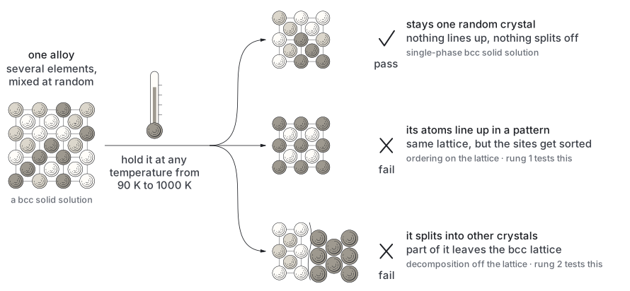
The first way to fail keeps every atom on the same grid of sites. Only who sits where changes. At high temperature the elements are scattered at random; on cooling, if the atoms of one element gain energy by having atoms of another as neighbours, they begin to prefer those neighbours (short-range order, chapter 3), and below a definite temperature the preference locks into a pattern that runs through the whole crystal (an order–disorder transition, chapter 4). Chapters 5 to 7 are about how to compute that temperature.
The second way to fail abandons the lattice. The alloy may be lower in energy as a mixture of other structures, for example a Laves phase, a compound with its own crystal that the bcc lattice cannot represent. A model that only knows the bcc lattice cannot see this competitor at all, which is why it gets its own rung and its own chapter (chapter 8).
A third question decides whether either failure matters in practice: whether the atoms can move far enough, at the temperatures in the window, for the change to happen at all within a part's life. That is kinetics, chapter 9.
One gap is stated rather than hidden. Chromium on its own turns antiferromagnetic at 311 K, inside the window, and every rung of the nine-element ladder computes energies without electron spin (E122). A composition containing chromium is flagged for that reason; no rung can tell what alloying does to that transition.
Where the idea comes from
That the order–disorder temperature of these alloys can be moved by composition, and by a lot, is a published result. Sobieraj and co-workers built a cluster expansion (a fast model of the alloy's energy, chapter 5) for the Cr–Ta–Ti–V–W family from first-principles energies, and cooled it by Monte Carlo (a simulated slow cooling, chapter 7) (Sobieraj et al., Phys. Chem. Chem. Phys. 22, 23929, 2020). The equiatomic Cr–Ta–V–W alloy orders at 1300 K, and adding titanium pulls the temperature down:
| titanium added | ordering temperature |
|---|---|
| none (equiatomic Cr–Ta–V–W) | 1300 K |
| 10 % | 1000 K |
| 40 % | 800 K |
| 50 % and above | 300 K |
Composition is a lever on exactly the quantity this requirement is about.
The published record also says the requirement is hard. Of the twelve published order–disorder temperatures this project collected for alloys of these elements, seven fall inside 90–1000 K (E150). Most well-known compositions fail.
How this project answers it
Nobody can cast and test thousands of alloys to find the few that pass, so the question is answered by computation, in steps of rising cost. The cheapest step estimates the energy of the random alloy (chapters 5 and 6). The next cools a model of the alloy slowly and watches for a transition (chapter 7). Then come the off-lattice competitors, the kinetics, and finally a quantum-mechanical calculation on a few dozen atoms (chapters 8 to 10). Each step is a rung; together they are the fidelity ladder of chapter 11, and each rung only sees compositions the rung below let through.
The compositions are proposed by a generator, a swarm of searchers steered by a readout on the wiring diagram of a fly's brain, which learns from the ladder's verdicts (chapter 12). For each composition the ladder returns a probability that it holds one phase across the window, not a yes or a no.
The latest walk up the ladder took the 32 compositions an earlier search had found and put them through the first three rungs, 0 to 2, on the current model; 11 passed (E240). Three independent models were then asked to agree on one of them, and they picked Mo₅₁Ti₃₈W₃Ta₃ (E241). Whether it truly does not order is being tested at the top rung, in E242.
Chapter 13 reports what the ladder found. The record of how the project got here, including what it tried and abandoned, is in the Logbook.
Chapter 2
Atoms on a lattice
Picture an egg box that goes on in every direction, with an egg in every cup. Metal atoms in a crystal sit like that: on a regular grid of places, each place the same as every other, repeated through the whole piece. The grid is the lattice and each place on it is a site. Everything in the next five chapters happens on one such grid.
The body-centred cubic lattice
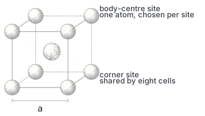
The lattice these metals share is the simplest one after a plain stack of cubes. Take a cube, put an atom at each corner, and put one more in the middle. Stack such cubes in every direction. That is the body-centred cubic lattice, bcc for short. The edge of the cube is the lattice constant, \(a\); for these alloys it is about 3.2 Å, a third of a billionth of a metre (the ordered cells in the training data of chapter 6 have a median of 3.23 Å, E149).
Each atom has eight nearest neighbours, at the corners of the cube around it, at a distance of \(\sqrt{3}\,a/2\). The next six sit one cube edge away, at \(a\). The two shells lie close together, at \(0.87\,a\) and \(a\), so an atom feels both sets of neighbours strongly, and both carry information about which neighbours it prefers (chapter 3).
A corner atom and a centre atom are not different kinds of site. Shift the grid by half a cube along its diagonal and the centres become corners. Every site of a bcc lattice is equivalent to every other. That will stop being true the moment the atoms order: in the ordered pattern called B2, one element takes the corners and another the centres, and the two sets of sites become distinguishable (chapter 4).
Which metals are bcc
The nine elements form a compact block of the periodic table: titanium, zirconium and hafnium in group 4, vanadium, niobium and tantalum in group 5, chromium, molybdenum and tungsten in group 6. Elements in one group have the same number of outer electrons and tend to behave alike, a similarity the model of chapter 6 learns on its own.
Molybdenum, niobium, tantalum, tungsten, vanadium and chromium are bcc at every temperature up to melting. Titanium, zirconium and hafnium are not: as pure metals they are hexagonal at room temperature and become bcc only when hot, at 1155, 1136 and 2013 K respectively (E122). In an alloy with enough of the first six they can be held on the bcc lattice. Whether a given titanium-rich alloy would rather leave it is exactly the off-lattice question of chapter 8.
A solid solution
Now fill the egg box with eggs of nine colours, poured in at random. Each cup still holds one egg; only the colour at each cup is left to chance. That is a solid solution: several elements sharing the sites of one lattice, each site taken by whichever atom landed there. Because one atom substitutes for another on the same site, it is called a substitutional solid solution, and when the elements are mixed with no preference for any neighbour it is a random solid solution.
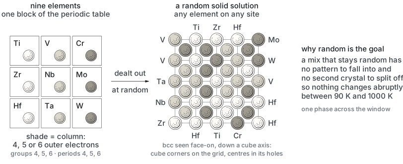
In the language of the rest of the book, one colouring of the lattice is a configuration, or decoration: a list of which element sits on which site. A composition, such as half molybdenum and half tantalum, fixes how many of each colour there are. It does not fix where they go, and there are an astronomical number of ways to place them. For the 432-site cell used in chapter 7, a 50/50 binary alone can be arranged in \(\binom{432}{216}\) ways, a number with about 129 digits.
Why many elements mix
Conventional alloys are one base metal with small additions. In 2004 Yeh and co-workers, and independently Cantor and co-workers, reported that alloys of five or more elements in near-equal proportions often form a single solid solution, not the tangle of compounds a phase diagram would suggest (Yeh et al., Adv. Eng. Mater. 6, 299, 2004; Cantor et al., Mater. Sci. Eng. A 375–377, 213, 2004). Yeh named them high-entropy alloys. In 2010 Senkov and co-workers made the refractory version: equiatomic W–Nb–Mo–Ta and W–Nb–Mo–Ta–V, cast by arc melting, each a single bcc solid solution (Senkov et al., Intermetallics 18, 1758, 2010). MoNbTaW and MoNbTaVW recur throughout this project's record as test cases.
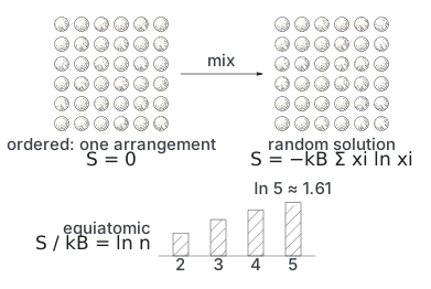
The name points at the reason. Nature counts arrangements. A random mixture of many elements can be made in many more ways than an ordered one, and at a finite temperature the number of ways is worth something, like energy. That worth is the configurational entropy. For an ideal random mixture with a fraction \(x_i\) of element \(i\), it is, per atom,
where \(k_B\) is Boltzmann's constant. For \(n\) elements in equal amounts it is \(k_B\ln n\). The logarithm grows slowly, so going from four elements to nine adds much less than going from one to four.
Energy against entropy
Whether the alloy stays mixed is a contest between two things. The energy (strictly, the enthalpy) says which neighbours the atoms prefer. The entropy, multiplied by the temperature, says how much disorder is worth. The quantity that decides is the free energy \(G = H - TS\), and the arrangement with the lowest \(G\) wins. At high temperature the \(TS\) term is large and the random mixture wins. At low temperature it shrinks and the energy decides.
That is why the cold end of the window is the hard end: at 1000 K entropy usually wins; at 90 K it usually does not. The two sides are compared below in meV per atom (a meV is a thousandth of an electronvolt, the energy scale of atomic arrangements):
| what is being weighed | meV per atom |
|---|---|
| mixing entropy's worth to an eight-component random solid solution at 1000 K (E56) | about 180 |
| the same at 90 K | about 16 |
| the energies that separate a random arrangement from an ordered one in these alloys | tens |
| the ordering spread measured directly in this project's training data (E151) | about 29 |
Something has to happen to the energy side for a solid solution to survive the cold, or it has to be unable to act on its preference in time (chapter 9).
The cells this project computes on
A computer cannot hold an infinite egg box, so every calculation uses a finite block of cubes repeated periodically: what leaves one face comes back in through the opposite one. Each kind of calculation uses its own block:
| calculation | block of cubes | atoms |
|---|---|---|
| the Monte Carlo of chapter 7 | 6 × 6 × 6 | 432 sites |
| the quantum-mechanical calculations of chapter 10 | 3 × 3 × 3 | 54 |
| the training data of chapter 6 | various | 2 to 128 |
A composition is placed on a cell by giving each element its share of the sites, rounded to whole atoms, and then choosing which sites at random.
Chapter 3
Short-range order
Watch a room fill up at a party where half the guests come from one group and half from another. If nobody cared who they stood next to, a guest's neighbours would be half from each group, give or take. If the two groups get on unusually well, each guest ends up with more neighbours from the other group than chance would give. There is no seating plan, but look at any one guest and the neighbours are not random.
That is short-range order. It is a preference visible in the neighbourhood of each atom, without any pattern that runs across the whole crystal.
Counting neighbours against chance
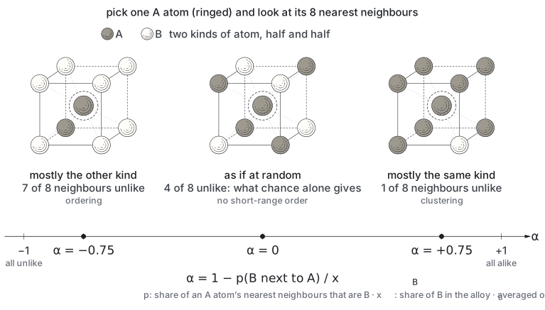
Take a random solid solution on the bcc lattice, pick an atom of element A, and look at its eight nearest neighbours. If the alloy is truly random and a fraction \(x_B\) of all atoms are B, then on average a fraction \(x_B\) of those eight will be B. Now suppose A and B lower the energy when they sit together. At high temperature the preference barely shows; as the alloy cools, A atoms collect more B neighbours than \(x_B\) would give. The excess is local: nothing about it requires the A atoms to line up with each other across the crystal.
To measure it, count. For every A atom, note what fraction of its neighbours in a given shell are B, average over all A atoms, and compare with \(x_B\). That comparison, turned into a single number per pair of elements and per shell, is the short-range order parameter.
The Warren–Cowley parameter
The number was introduced by J. M. Cowley in 1950, in a theory of order in alloys that he compared with what X-ray diffraction was then measuring, copper–gold alloys among them (Cowley, Phys. Rev. 77, 669, 1950). Cowley defined one parameter \(\alpha_i\) for each shell \(i\) of neighbours around an atom and related them to the interaction energies and the temperature; the long-range order of chapter 4 appears in his theory as the limit of very distant shells. The parameters are usually called Warren–Cowley parameters. For a pair of different elements \(A\) and \(B\) and one shell,
where \(p_{B\mid A}\) is the fraction of an A atom's neighbours in that shell that are B, and \(x_B\) is the fraction of B in the whole alloy.
Read it in words. If A's neighbours are B exactly as often as chance gives, \(p_{B\mid A}=x_B\) and \(\alpha=0\). If they are B more often, \(\alpha\) is negative: A and B prefer each other, and the alloy is leaning towards order. If they are B less often, \(\alpha\) is positive: A avoids B, and A atoms are leaning towards clustering with their own kind, the first step towards the alloy separating into regions.
The parameter has a floor. A cannot have more than all of its neighbours be B, so \(\alpha_{AB}\ge 1-1/x_B\), and because the count is symmetric between the two elements, \(\alpha_{AB}=\alpha_{BA}\) and the floor is the larger of \(1-1/x_A\) and \(1-1/x_B\). It is reached only by perfect order. In a 50/50 binary that floor is \(-1\): every A surrounded entirely by B, which on bcc is the B2 pattern of chapter 4.
Both statements, symmetry and floor with equality only for perfect order, are proved by this project in Lean 4, a program that checks every step of a proof, and the proof is tied to a test of the function that computes \(\alpha\) (formal/, WarrenCowley).
Shells beyond the first
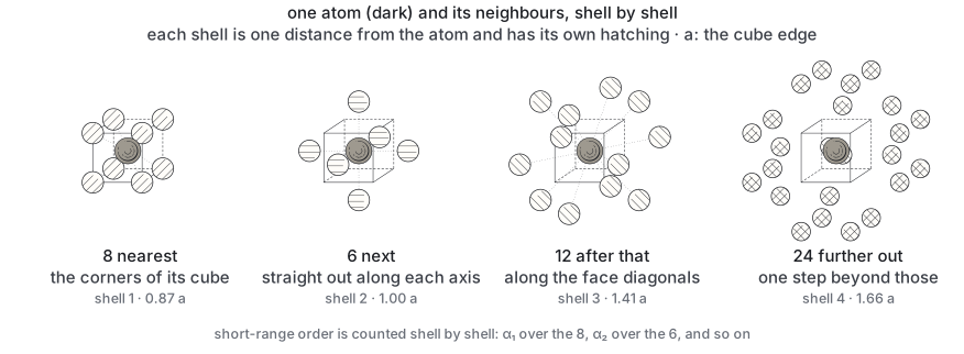
Around any bcc site the neighbours come in shells: 8 at the cube diagonal, 6 one cube edge away, 12 across a cube face, 24 further out. The shells tell different things. When unlike atoms prefer to be nearest neighbours on bcc, the second shell, which in the B2 pattern holds atoms of the same kind, shows the opposite sign.
The outer shells are also a diagnostic of the energy model. Even a model with only nearest-neighbour interactions produces some order in outer shells, carried outward by the inner ones. So a model's outer-shell order is judged against that induced baseline.
Measured this way, this project's previous model (v5) was nearest-neighbour plus a real second-shell interaction, and nothing further (E220). At 3000 K its ratio of second-shell to first-shell order was −0.50, against −0.22 for a model with nearest-neighbour interactions only. Its third and fourth shells stayed close to the induced values, and matched them at 1550 K.
Why it matters
Short-range order is the forerunner of order. Above an order–disorder transition the local preference is already there, and it grows as the alloy cools until it locks into a pattern through the whole crystal: the transition of chapter 4.
It also costs entropy. Any preference reduces the number of arrangements the alloy actually visits. Kim and Widom computed how much for equiatomic Mo–Ta and MoNbTaW and found that above the transition the loss is modest, less than 20 % of the ideal value, about \(0.1\,k_B\) per atom for Mo–Ta (Kim & Widom, Phys. Rev. Materials 7, 063803, 2023). Below the transition it drops rapidly.
And it is what an experiment can see. Cowley's parameters were made to be compared with the diffuse scattering of X-rays, which is how short-range order is measured in a real alloy.
How this project measures it
This project's Monte Carlo (chapter 7) computes \(\alpha\) directly from the configuration: for each unlike pair of elements and each of the four shells, it counts neighbours on the 432-site cell and applies the formula above. Alongside each ordering temperature it reports one pair: the strongest ordering pair at the coldest point of the run, with its first-shell \(\alpha\).
For equiatomic Mo–Ta on the shipped model that pair is Mo–Ta, and on cooling \(\alpha_1=-1.00\) (E242). That is perfect B2, at the floor the formula allows.
In a many-element alloy the floor sits lower, and values below \(-1\) are allowed. With a quarter each of four elements, the floor for any pair is \(1-1/0.25=-3\). On the previous model, equiatomic Cr–Ta–Ti–W cooled to a first-shell Cr–Ta \(\alpha_1\) of \(-1.03\). In words: about half of each chromium atom's neighbours were tantalum, twice what chance gives, a strong preference well short of perfect order (E210b).
A finite cell limits what can be read. On 432 sites, an element with only a handful of atoms has only a handful of neighbours to count, and its \(\alpha\) is mostly noise. Two lone atoms of different elements that happen to touch can read \(\alpha=-53\).
So a pair is reported only if its \(\alpha\) is readable on the cell. In plain terms, chance alone must not be able to fake the reading, and perfect order must stand clear of chance. The rule has two parts:
- the standard error of \(\alpha\) must be at most 0.1;
- the pair's floor must lie more than three standard errors below the random value.
The rule was derived exactly for a random decoration of fixed counts and checked against exhaustive enumeration on 18 small lattices. Its practical effect: an element below about 7 % of the cell, 30 atoms, cannot show detectable order even when perfectly ordered, and its pairs report nothing (E240). The ordering temperature itself does not depend on this choice.
Reading pyeCE's own column
pyeCE, the embedded-cluster-expansion library this project trains its model with (chapter 6), has its own Monte Carlo, which writes a short-range-order column per pair. Under the aggregation setting this project's runs used (reduce: true), that column is not \(\alpha\). It mixes \(\alpha\) with a second number and has to be decoded before it can be read.
The library averages two numbers it has computed, \(\alpha\) and its standard deviation \(\sigma\) over the samples, as if they were two samples of one quantity. So the column holds \((\alpha+\sigma)/2\), and its interval has half-width \(t\,|\alpha-\sigma|/2\) with \(t=12.706\), the two-sample Student-\(t\) factor.
Both numbers are recovered exactly. For an ordering pair, \(\alpha<0\le\sigma\), so \(\alpha\) is the lower of the two. For a pair with \(\alpha>0\) the two cannot be told apart from the file, and nothing is reported (E216).
Decoded, pyeCE's values agree with this project's sampler to within 0.007 at every temperature compared. The decoding is proved in Lean and pinned by a test. How the encoding was found is told in the Logbook.
Chapter 4
When order appears
Take a tray of black and white marbles in a shallow grid, and suppose each black marble would rather have white neighbours. Shake the tray hard and the marbles land anywhere; the preference is swamped. Shake it gently and something different happens: a checkerboard patch forms, then another, and at some gentleness the patches join up into a single checkerboard across the whole tray. Between hard and gentle there is a point where the tray changes character, from a random scatter with local preferences to one pattern everywhere.
Temperature is the shaking. The point where the pattern takes over is the order–disorder transition.
Long-range order
Short-range order (chapter 3) is about each atom's neighbours. Long-range order is about the whole crystal. In the ordered state the lattice splits into two or more interpenetrating sets of sites, called sublattices, and each element keeps mostly to its own. Knowing which element sits on one site then tells you, with better than chance odds, which element sits on a site a thousand atoms away.
On the bcc (body-centred cubic) lattice the simplest such pattern is B2. Recall from chapter 2 that the cube corners and the cube centres form two sets of sites. In B2 one element takes the corners and the other the centres, so every atom's eight nearest neighbours are of the other kind. This is the CsCl structure; in equiatomic Mo–Ta it means every molybdenum surrounded by eight tantalum atoms and every tantalum by eight molybdenum.
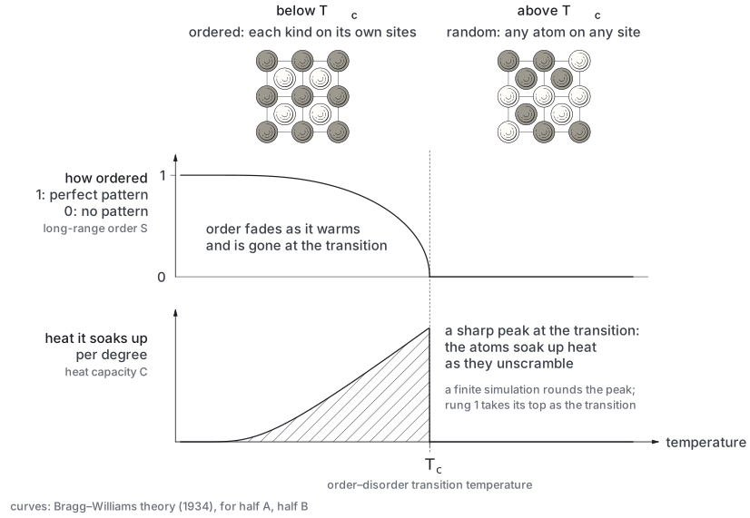
The amount of long-range order is measured by an order parameter, usually written \(S\). It is 1 when every atom is on its own sublattice, 0 when the sublattices are indistinguishable, and in between it measures how much better than chance the sorting is. Above the transition \(S=0\); below it \(S\) grows as the crystal cools.
Where the idea comes from
The theory of this transition was set out by W. L. Bragg and E. J. Williams in 1934 (Bragg & Williams, Proc. R. Soc. Lond. A 145, 699, 1934). Their argument is a feedback loop. The energy an atom pays for sitting on the wrong sublattice depends on how ordered its surroundings are, which is to say on \(S\) itself. So the more ordered the crystal, the stronger the push towards more order. At low temperature the feedback wins and \(S\) is large; as the temperature rises, thermal agitation wins a little more at each step, and at a critical temperature \(T_c\) the ordered solution disappears and \(S\) falls to zero.
Bragg and Williams made one simplifying assumption: each atom feels only the average order of the whole crystal, not the actual atoms around it. That is a mean-field theory. It ignores short-range order, the local preferences that survive above \(T_c\) and make the disordered state cheaper than a truly random one. Without them disorder looks more costly than it is, and mean-field theory puts the transition too high.
A model with a known answer shows by how much. This project's known-answer model is nearest-neighbour bcc with \(J=19.12\) meV per bond (a meV is a thousandth of an electronvolt) (E215). Its exact transition is at 1410 K; the mean-field estimate, \(8J/k_B\), is about 1775 K. Cowley's theory of chapter 3 was one of the attempts to add the short-range part back.
One consequence of the Bragg–Williams picture holds well beyond its approximations: the transition temperature is proportional to the energy the order gains. Double the ordering energy and \(T_c\) roughly doubles.
This project uses that proportionality as an estimate, never as a measurement. One example: the previous model over-ordered the chromium–tantalum pair in Cr–Ta–Ti–W. A quantum-mechanical calculation (density functional theory, DFT, chapter 10) found that pair's ordering energy to be 44.9 meV per atom, against 107.9 in the model. Scaling the model's 1461 K by that ratio puts the transition near 600 K, within one grid step of a published 500 K (E222).
The signature in the heat capacity
How do you see a transition in a calculation or in a measurement? By the heat it absorbs. Warming an alloy through \(T_c\) costs extra energy, because the arrangement is coming apart and every broken preference is energy taken up. So the heat capacity, the energy needed to raise the temperature by one kelvin, has a peak at \(T_c\).
In a Monte Carlo simulation the heat capacity can be read two ways. One is the slope of the mean energy against temperature, \(C=\mathrm{d}\langle E\rangle/\mathrm{d}T\). The other is the size of the energy's fluctuations at one temperature,
In equilibrium the two are the same quantity, and chapter 7 reads both. Near \(T_c\) the fluctuations are large because the alloy wavers between ordered and disordered patches.
The precise name for \(T_c\) in this setting is the order–disorder transition temperature, \(T_{\mathrm{od}}\) in this book and ODTT in some papers. For the B2 transition on bcc it is continuous: \(S\) goes to zero smoothly rather than jumping, and Kim and Widom confirm that for Mo–Ta and MoNbTaW it belongs to the same class as the three-dimensional Ising model of magnetism (Kim & Widom, Phys. Rev. Materials 7, 063803, 2023).
Comparing with published numbers
A transition temperature is only comparable with another if both are the same observable, on the same kind of lattice. Published values for these alloys come as heat-capacity peaks, susceptibility peaks, inflections of the enthalpy of mixing, free-energy crossings and stability limits of the disordered state. For a continuous transition the first three estimate the same critical temperature; the last two do not. This project keeps a table of published values with each row's observable, lattice convention and spin treatment, and compares only like with like (forager/ladder/published_odt.py).
That rule is why one published definition had to be read in the source. Sobieraj and co-workers define their temperature as the highest temperature at which the enthalpy of mixing, plotted against temperature, has an inflection (Sobieraj et al., Phys. Chem. Chem. Phys. 22, 23929, 2020). At fixed composition that enthalpy differs from the Monte Carlo energy by a constant, so its inflection is a heat-capacity peak, and their values are comparable with this project's.
How this project uses it
Rung 1 of the ladder asks one question: does this composition have an order–disorder transition inside 90–1000 K? It answers by cooling the model alloy (chapter 7) and locating the heat-capacity peak.
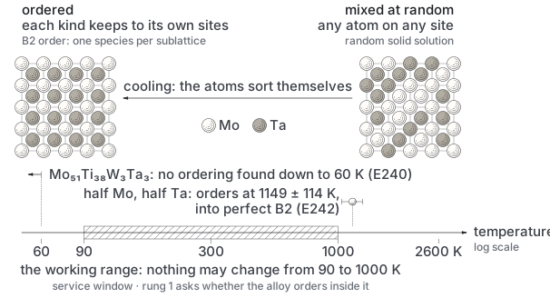
The known answer the shipped model must reproduce is equiatomic Mo–Ta. The requirement set before the run was a transition between 500 and 2600 K, and the model meets it: through the production path it orders at 1149 ± 114 K, into perfect B2, \(\alpha_1=-1.00\) (E242). The published value is higher, and itself uncertain:
| Mo–Ta transition | value |
|---|---|
| shipped model, production path | 1149 ± 114 K |
| previous model, same sampler | 985 K |
| Kim and Widom's susceptibility peak (published) | 2020 K |
| error that published number carries from its own model error of 21 meV per atom (this project's estimate) | about ±545 K |
The method was scored against the published table on the previous model, v5, before the shipped model existed. Of seven systems with a comparable published value, six fell within 22 % of it. The seventh was Cr–Ta–Ti–W, at 2.92 times the published value: the over-ordered chromium–tantalum pair above, which DFT confirms does order, but less strongly (E210b, E222).
The same table is where chapter 1's warning comes from: of the twelve published temperatures for alloys of these elements, seven lie inside the window (E150).
Chapter 5
The energy of an arrangement
Suppose you had to score seating plans for a dinner. You know, for every pair of guests, how well they get on sitting side by side, and you have a few corrections for particular trios. To score any plan you walk round the table, add up the number for every pair of neighbours, add the trio corrections, and you have the evening's total. You never have to hold the dinner to know how it would go. And if you swap two guests, you only need to rescore the seats around those two.
The energy of an arrangement of atoms on a lattice can be scored the same way. That is the idea of this chapter.
A sum over small groups of sites
On a fixed lattice, an alloy's configuration is just the list of which element sits on which site (chapter 2). Its energy depends on that list and nothing else. The cluster expansion writes that energy as a sum of contributions from small groups of sites, called clusters: single sites, pairs of sites at each neighbour distance, triangles of three sites, and so on. Each kind of cluster carries a number, its weight, which says how much it contributes when particular elements occupy it.
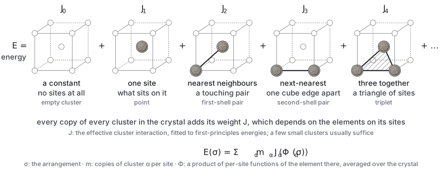
Written out, with the words first: the energy of configuration \(\sigma\) is a constant, plus a term for each kind of site, plus a term for each kind of pair, plus a term for each kind of triangle, and so on, each term being a weight times how the elements are arranged on all clusters of that kind:
Here \(\alpha\) runs over the distinct kinds of cluster (all pairs at the first-neighbour distance are one kind, all at the second another), \(m_\alpha\) counts how many clusters of that kind there are per site, \(J_\alpha\) is the weight, called the effective cluster interaction, and \(\langle\Phi_\alpha(\sigma)\rangle\) is a number describing which elements sit on clusters of that kind, averaged over all of them in the crystal, the correlation function. For two elements the correlation function of a nearest-neighbour pair is just a signed count of like against unlike nearest neighbours, which is why it is so closely tied to the short-range order of chapter 3.
Where the idea comes from
The general form for any number of elements was given by J. M. Sanchez, F. Ducastelle and D. Gratias in 1984 (Sanchez, Ducastelle & Gratias, Physica A 128, 334, 1984). Their contribution was to describe what sits on a cluster through an orthogonal set of functions of the site occupations, so that the correlation functions form a complete, independent set: with every cluster included, the expansion can represent any energy that depends only on the configuration. In practice the weights fall off quickly with the size and extent of the cluster, so a handful of pairs and a few triangles carry nearly all of it, and the series is cut there.
The weights are not computed from first principles one by one. They are fitted: compute the energies of a few hundred or a few thousand arrangements with a quantum-mechanical method (chapter 10), and choose the weights that reproduce them. The fitted expansion then predicts the energy of arrangements nobody computed.
Why it is the right tool here
The point of the expansion is speed. Once the weights are known, the energy of any arrangement is a sum, and the change in energy when two atoms swap places only involves the clusters that touch those two sites. That makes it possible to try millions of swaps and let an alloy find its preferred arrangements at each temperature, which is what the Monte Carlo of chapter 7 does. A quantum-mechanical calculation of one 54-atom cell takes more than an hour on a large graphics card (chapter 10); the expansion prices a swap in under a millisecond.
Smearing the atoms
A DFT calculation (density functional theory, chapter 10) meets a similar problem with electrons. An electron state is either occupied or empty, a sharp step, and a step makes the energy jump. DFT codes smear the step into a smooth function, and the energy becomes smooth too.
The operator of this project proposed the same trick for atoms (E34). Smear which element sits on a site: let a site be part titanium and part tungsten, say. The cluster expansion still returns an energy, and that energy now changes smoothly from one arrangement to another instead of jumping.
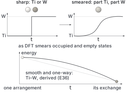
The same construction also links two numbers this project uses, if every site is smeared toward the alloy's overall composition instead of toward a swapped arrangement. Unsmeared, the energy is that of one fixed arrangement. Smeared all the way, each site holds each element in proportion to the composition, independently of its neighbours, and for a cluster expansion the energy is exactly that of the random solid solution, the number rung 0 estimates (chapter 6). In between, the sites keep part of the arrangement's pattern, like a partly ordered crystal in the Bragg–Williams picture of order. What smearing cannot hold is short-range order (chapter 3). Short-range order is a correlation between neighbouring sites, and sites smeared independently carry none.
The smeared energy can be derived rather than sampled (E36). Each cluster touches at most three sites, and each site contributes a factor linear in the smearing, so the energy is a cubic in the smearing parameter however many sites are smeared.
The worry was that a site half hafnium, half tungsten is too unphysical to smooth anything. On a 16-site cell it was not. Of eight paths exchanging one element for another, seven are monotone, with no turning point, including every pair spanning groups 4 to 6; the eighth, Ti–Zr, turns once. A path between two arrangements is weaker evidence than smoothness of the whole landscape.
The method is published: Kaappa, Larsen and Jacobsen interpolate between chemical elements to optimise structure and ordering, shown on Au–Cu and Cu–Ni, neighbours in the periodic table (Kaappa, Larsen & Jacobsen, Phys. Rev. Lett. 127, 166001, 2021). The operator reached it independently; what E36 adds is the test across groups 4 to 6.
What it cannot do
The expansion knows the lattice and the occupations, and nothing else. That has three consequences, and each shapes a later chapter.
It has no notion of atoms being pushed off their sites, or of the crystal swelling and shrinking with composition. Real atoms in an alloy sit slightly off the ideal sites, and each composition has its own lattice constant; an expansion cannot represent either, so it must be trained on energies from which those effects have been removed.
In this project's training data those effects are far larger than the signal the expansion has to learn. In meV per atom (a meV is a thousandth of an electronvolt), from E150:
| energy in the training data | meV per atom |
|---|---|
| atoms pushed off their sites (displacement), on average | about 200 |
| cells squeezed or stretched (volume), at most | about 1700 |
| the ordering signal the expansion must learn | 10 to 30 |
Removing them correctly is the label correction of chapter 6.
It cannot see a competitor that lives on a different lattice. A Laves phase has its own crystal; an expansion on the bcc (body-centred cubic) lattice has no configuration that looks like it, so it can never lose to it. It will return a confident ordering temperature for a composition whose real ground state is something else entirely. That is why rung 2 exists (chapter 8).
And it grows quickly with the number of elements. With \(K\) elements, each site is described by \(K-1\) functions, so a pair cluster carries \((K-1)^2\) correlation functions and a triangle \((K-1)^3\), before symmetry trims them. For two elements that is one of each. For nine it is 64 per kind of pair and 512 per kind of triangle, each needing its own weight and enough training data to pin it. Sanchez's framework handles any number of elements in principle; in practice conventional cluster expansions have mostly been limited to three or four (Müller & Natarajan, npj Comput. Mater. 11, 60, 2025). Chapter 6 is about how that limit is lifted.
How this project uses it
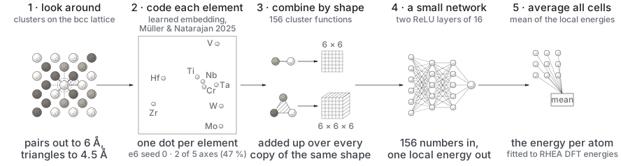
This project's energy model is an embedded cluster expansion (chapter 6), a cluster expansion in the sense of this chapter whose site functions are compressed and whose weights are replaced by a small neural network. Its clusters are pairs out to 6 Å, which on the bcc lattice of these alloys covers the first five neighbour shells, and triangles out to 4.5 Å.
Longer pairs were tried and did not help where it mattered. A test arm with pairs out to 10 Å, fifteen shells, improved the model's error on everything except the one quantity it was meant to fix, the molybdenum–tantalum ordering energy (E233). So the range stayed at 6 Å for the model that ships.
One caution comes with periodic cells, and it was checked. The expansion is evaluated on a periodic cell of 432 sites (chapter 7). If a cluster reaches further than half the cell, it can meet a periodic copy of its own atoms. The cell's edge is 6 cubes, about 19.8 Å, so the test arm's 10 Å pairs exceed half of it. The shipped model's 6 Å pairs are well inside the limit in any case.
Whether the energy is still right with 10 Å pairs was tested against a known answer. A pattern that repeats every 3 cubes must have the same energy per site whether it is computed on its own 3-cube cell or tiled onto the 6-cube cell. It does, to 0.000015 meV per atom, because the library counts every lattice vector once instead of folding it back to the nearest copy (E237, the exact-evaluator review).
The first bottom rung of this project was a conventional cluster expansion fitted to a machine-learned potential's energies at one fixed lattice constant. How it was tested against first-principles data and replaced is told in the Logbook.
Chapter 6
Learning the expansion
A screen does not keep a name for every colour. It describes each by three numbers, how much red, green and blue, and every shade becomes a point in a small space where similar colours sit close together.
The embedded cluster expansion does the same for chemical elements.
Nine elements in a few numbers
Chapter 5 ended on a count: with nine elements, a conventional cluster expansion needs 64 correlation functions for every kind of pair and 512 for every kind of triangle. The embedded version replaces each element's fixed set of site functions by a short list of learned numbers, its code. The cluster functions are built from the codes, so their number grows with the length of the code, not with the number of elements. A small neural network then turns the cluster functions around each site into a local energy, and the local energies are averaged into the energy per atom.
The codes are learned from the energies, and they pick up chemistry without being told any: elements that behave alike end up with nearby codes.
Where the idea comes from
The embedded cluster expansion was introduced by Y. L. Müller and A. R. Natarajan (npj Comput. Mater. 11, 60, 2025). They tested it on a six-element alloy of V, Nb, Ta, Cr, Mo and W. Codes of three numbers reproduced the energies to within 4 meV per atom (a meV is a thousandth of an electronvolt). The harder test was a pair of elements the model had never seen: it predicted that pair with an average error of about 8 meV per atom, against about 30 for a conventional expansion. Codes of three or four numbers extrapolated best; longer ones did worse.
Their library, pyeCE, which this project trains with, followed with one model for a nine-component refractory alloy on the same nine elements (Müller, Paetsch & Natarajan, arXiv:2609.10190, 2026).
The training data
The energies come from the RHEA (refractory high-entropy alloy) database of J. Byggmästar and co-workers, published openly (Byggmästar, Lopes, Fan & Ala-Nissila, arXiv:2603.04147, 2026; data at doi:10.5281/zenodo.18863415). It holds 22,477 structures of the same nine elements, computed with density functional theory (DFT, chapter 10): the VASP code (Vienna Ab initio Simulation Package), the PBE (Perdew–Burke–Ernzerhof) functional, no spin polarisation. The groups used here are 4,750 ordered bcc (body-centred cubic) cells, 2,150 random 54-atom solid solutions and 1,608 random binaries (E149).
The database was built to train interatomic potentials, so its atoms are deliberately pushed off their sites and its cells deliberately squeezed and stretched. Across the cubic bcc cells, atoms sit on average 0.13 Å off their ideal sites and lattice constants range from 2.665 to 3.818 Å (E150). A cluster expansion cannot represent either (chapter 5). The raw energies are not labels it can learn from.
Labels a lattice model can learn from
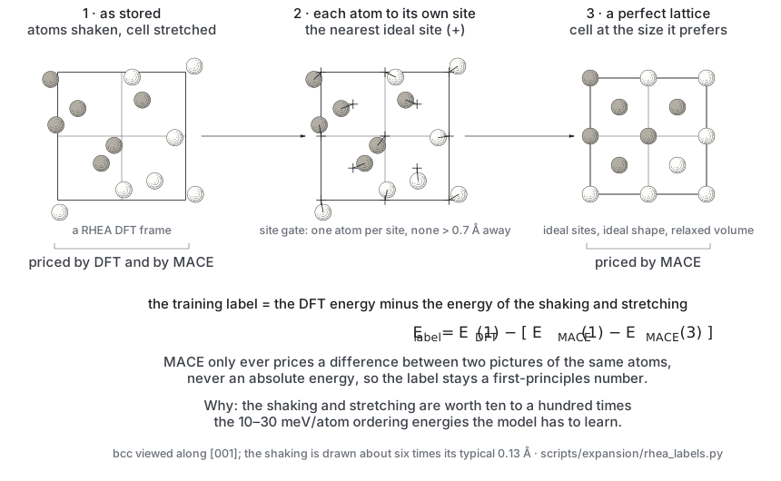
The fix subtracts what the lattice model cannot see:
In words: ask a machine-learned potential (MACE, chapter 8) how much energy the displacements and strain add to this very cell with these very atoms, and remove it from the DFT energy. The potential only supplies a difference on one structure, so the label stays a first-principles number.
Each part was checked against something it could fail.
The potential is not soft on these frames, meaning it does not systematically under-report forces. Across 150 of them its forces match DFT's with a slope of 1.014 and its pressures with 1.072 (E228).
The lattice minimum has to be the true minimum. A parabola fitted over ±10 % in lattice constant had put it 0.047 Å too wide on average, which put every label 17.2 meV per atom too high. It is now found by a direct one-dimensional minimisation (E228, E231). A machine-checked proof in formal/ shows that inside the searched range such a miss can only raise a label, never lower it.
Frames sampled far from their own minimum carry more correction error, so the labels keep only frames within 0.10 Å of it: 4,326 frames, 97 % of the ordered cells.
The error that remains is 12.4 meV per atom, against an ordering spread of about 29 meV per atom (E151). It was measured where it should be zero: among random decorations of one composition, which have almost no real spread.
The pure-element references
One part is still open: the energies of the pure elements, against which formation energies are measured. RHEA holds few pure bcc frames of some: three for titanium; twelve for hafnium, spread over 34 meV per atom. So there are two defensible choices of reference, the lowest frame or the median frame, and they differ:
| element | gap between the two references, meV per atom per unit fraction |
|---|---|
| Ti | 33.5 |
| Cr | 28.1 |
| Hf | 22.0 |
The shift is linear in composition. It cancels in ordering energies, but it moves the absolute formation energies rung 0 scores. E239 measures it directly, by recomputing about 48 of RHEA's own ordered cells in Quantum ESPRESSO, a second DFT code (chapter 10).
One fit is not a model
Train one model three times, changing only the random seed. The three fits agree on random-like chemistry and disagree on ordered states, and the usual held-out score cannot see the difference (EXPERIMENTS.md, 22 September, the entry before E229):
| error, meV per atom | fit 1 | fit 2 | fit 3 |
|---|---|---|---|
| 48 held-out RHEA Mo–Nb–Ta–W cells | 7.2 | 7.4 | 7.5 |
| eleven DFT cells no model was steered towards | 22.9 | 16.6 | 23.8 |
On those eleven cells the three fits disagree about a single cell by 8.5 meV per atom on average, and by 25 on one ordered MoNbTaVW cell. Random-like chemistry is pinned down by the data; ordered states are not.
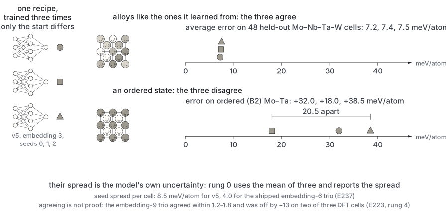
So rung 0 is never one fit. It is the mean of three, and every candidate model is judged as an ensemble on the eleven independent DFT cells and on three DFT cells from the search's own finds.
How many numbers per element
The length of the code decided the model. Short codes under-bind Mo–Ta's ordered B2 pattern (chapter 4); long codes fix ordered states but lose the chemical trends that carry an unseen composition. Scored as three-seed ensembles, in meV per atom (E237):
| code length | eleven DFT cells, mean error | B2 Mo–Ta error | held-out RHEA | search's random cells |
|---|---|---|---|---|
| 3 (previous model, v5) | 20.6 | +29.5 | 7.1 | 6.3 |
| 4 | 13.3 | +6.3 | 8.4 | 10.0 |
| 5 | 7.7 | +4.1 | 6.7 | 16.6 |
| 6 | 7.5 | −5.2 | 7.9 | 6.1 |
| 9 | 8.8 | +0.2 | 11.0 | 9.4 |
What the table shows, row by row:
- Nine numbers get the ordered B2 cell right and miss the search's random cells, confidently: off by 13 on two of the three, with a seed spread under 2 (E223).
- Five numbers pass every target set in advance, then miss one random cell, Mo₇₀Hf₂₀Ti₁₀, by 23.9 with a spread of 2.9.
- Six numbers hold both: the random cells as well as the previous model, and ordered states as well as nine.
This reproduces Müller and Natarajan's finding that longer codes extrapolate worse, with the best length a little longer than on their six elements.
The model that ships
The model that ships is the six-number, three-seed ensemble of E237. It was trained on the earlier labels: lowest-frame references, and the volume minimum before its refinement. Much of that miss cancels in formation energies, because the pure-element frames carry a similar one (E228).
A refit on the corrected labels did not meet its bar, so it does not ship. It used 5,836 rows, including 2,020 small ordered cells of non-cubic shape, and was tried in four versions. None held the search's random cells within the bar of 8 meV per atom: the best missed it at 13.6, the candidate at 19.6 (E238). A diagnostic traced the over-binding to the median Ti, Cr and Hf references, not to the new rows. So the fallback written before the refit applies until E239 sets the references.
Rung 0 uses the ensemble to estimate the energy of the random alloy. The estimate is the mean of the three members over eight random decorations of the composition; its uncertainty is their spread together with a 10 meV per atom model error. Rung 1 samples the same mean (chapter 7). The runs behind the choice are in the Logbook.
Chapter 7
Letting it cool
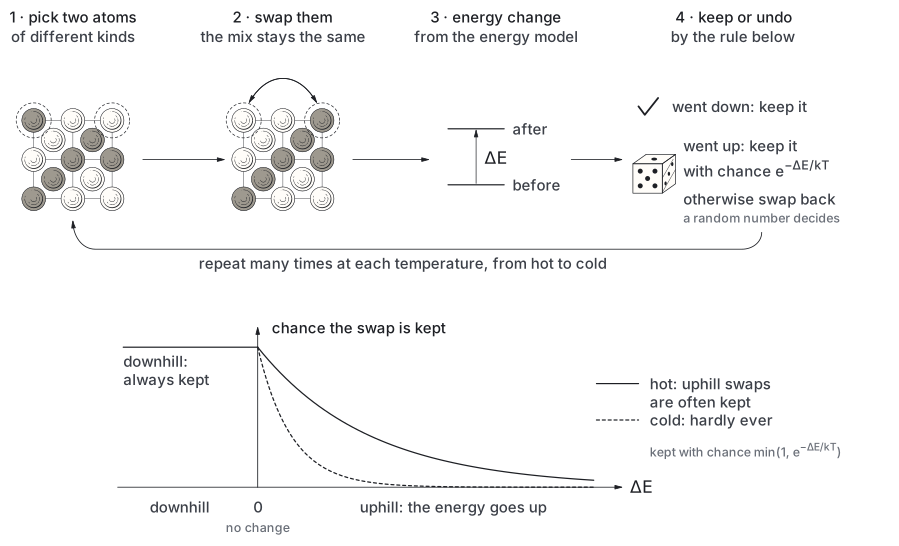
Imagine walking in fog over hilly ground, trying to spend time in each hollow in proportion to how deep it is. You cannot see the map, only the slope under your feet. So you use a rule: take a random step; if it goes down, keep it; if it goes up, toss a weighted coin and keep it only if the coin says so, with the coin more reluctant the steeper the climb. Walk long enough and your time is shared between the hollows in just the right proportion. Make the coin stingier and you settle into the deepest hollow you can reach.
That rule is how this project cools an alloy on a computer. The temperature sets how stingy the coin is.
The problem it solves
At a temperature \(T\), statistical mechanics says an alloy visits each arrangement \(\sigma\) with probability proportional to \(e^{-E(\sigma)/k_BT}\), the Boltzmann weight. Everything in chapters 3 and 4, the short-range order, the heat capacity, the transition, is an average over that distribution. But the number of arrangements is beyond counting: for a 50/50 alloy on 432 sites it has 129 digits (chapter 2). The average cannot be computed by listing them. It has to be sampled.
Where the idea comes from
The method was published in 1953 by N. Metropolis, A. W. Rosenbluth, M. N. Rosenbluth, A. H. Teller and E. Teller, who used it to compute the equation of state of 224 hard discs on the Los Alamos MANIAC computer (Metropolis et al., J. Chem. Phys. 21, 1087, 1953). Instead of drawing arrangements at random and weighting them, they built a chain of arrangements, each a small change of the last, accepted or rejected so that the chain visits each arrangement in proportion to its Boltzmann weight. A move that lowers the energy is always accepted; one that raises it by \(\Delta E\) is accepted with probability \(e^{-\Delta E/k_BT}\):
With this rule the flow from any arrangement A to any B exactly balances the flow back when the chain is in the Boltzmann distribution (detailed balance), so once there it stays there. This project's proof of detailed balance and stationarity for its own move is machine-checked in Lean 4, a program that checks every step of a proof. It is also tested on the exact transition matrix of a four-site lattice, to \(10^{-15}\) (formal/, DetailedBalance).
The swap move
The 1953 paper moved one particle at a time. For an alloy of fixed composition the natural move is a swap. Pick two sites; if they hold different elements, exchange them. The number of atoms of each element never changes, so the chain samples one composition, which is what an ordering temperature is a property of. The energy change of a swap is exactly what the cluster expansion of chapters 5 and 6 is built to price quickly.
How this project cools an alloy
Rung 1 places the composition at random on a periodic cell, starts hot, and cools it in steps, sampling at each one. The settings (E238 for the timing):
| setting | |
|---|---|
| cell | 432 sites, 6 × 6 × 6 bcc (body-centred cubic) cubes, atoms in random positions |
| temperatures | from 2600 K through twelve temperatures 227 K apart down to 100 K, then two more steps below the window's edge, to 80 and 60 K |
| at each temperature | 100 sweeps to let the alloy settle, 200 more to measure |
| one sweep | 432 attempted swaps of two sites chosen anywhere in the cell |
| cost | about 1.8 million swaps per composition, about 50 minutes on one processor core for the shipped model |
At every temperature it records the mean energy, its fluctuations and the short-range order of every readable pair (chapter 3).
The energy it samples is the mean of the three models in the shipped ensemble (chapter 6), so rung 0 and rung 1 score the same model.
A temperature that means what it says
The Boltzmann factor needs the change in the energy of the whole cell. The model outputs an energy per atom. This project's sampler multiplies the per-atom change by the number of atoms, so it samples at the temperature it reports.
pyeCE, the embedded-cluster-expansion library the model is trained with (chapter 6), has its own sampler, and it does something else: it samples at twice the temperature it reports. So a temperature read from pyeCE's sampler must be doubled.
The reason is bookkeeping. Its model outputs a per-atom energy for each two-site cell of the lattice, and its sampler adds up those outputs over the cells a swap touches. For two-site cells that sum is half the true change in energy. Accepting on half the energy at \(T\) is the same as accepting on the whole energy at \(2T\).
The factor was measured three independent ways:
| how it was measured | result |
|---|---|
| on the sampler's own swap bookkeeping, previous model | ratio exactly 0.500 |
| by a second sampler written from scratch (E216) | the same factor |
| on a transition known exactly (E215, E215c) | 2.000 ± 0.03 |
The identity between the two conventions is proved in Lean and tied to a test that fails if the factor is dropped. The story of finding it is in the Logbook.
An exact, faster evaluator
Pricing a swap through pyeCE's own neural-network code is slow for long codes. This project re-evaluates the same network exactly in plain numerical code, grouping the cluster functions by kind and folding the first network layer into them. It is the model computed another way, not an approximation, and at nine numbers per element it is 54 times faster than pyeCE (E237).
Checked on seven models, its energies match pyeCE's to 0.00000063 eV per cell and 0.023 meV per swap (an eV is an electronvolt; a meV is a thousandth of one). Its speed, in swaps a second:
| numbers per element | pyeCE's own code | exact evaluator |
|---|---|---|
| 3 | 1,009 | 2,788 |
| 4 | 1,987 | |
| 9 | 28 | 1,519 |
The acceptance test is parity of every swap, not agreement on one temperature. A fitted shortcut was also tried, and rejected. For Mo₄₂Ta₂₉Ti₂₉ it landed within 5 K of the model's own ordering temperature, while getting individual swaps wrong by 56 meV (root mean square). A number can be hit by accident. Every swap cannot.
Reading the transition from two channels
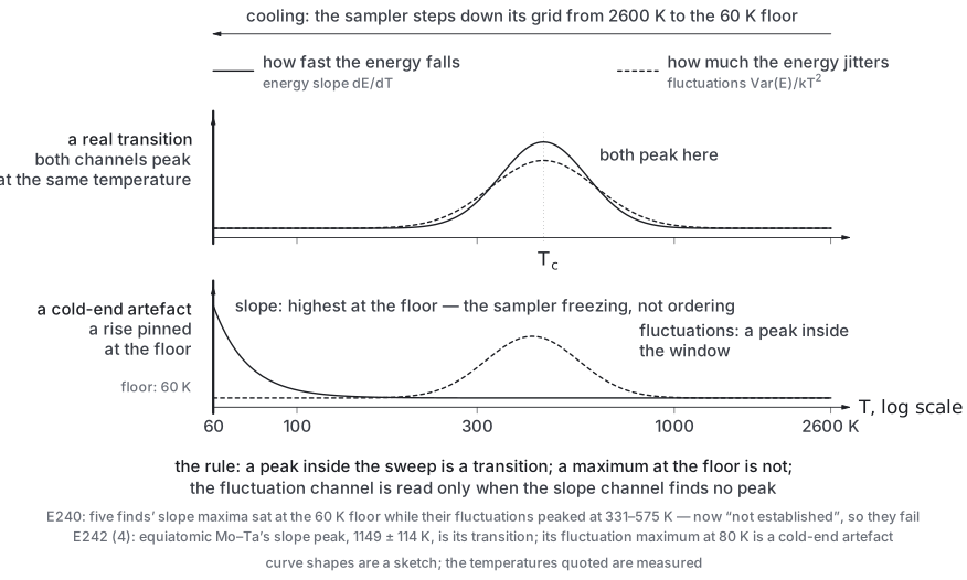
Chapter 4 gave two ways to read the heat capacity: the slope of the mean energy, and the fluctuations at one temperature. Rung 1 computes both from the same run. The transition is placed at the peak of the energy-slope channel, refined by a parabola through the highest points. Its uncertainty is half a grid step, 114 K in the hot part of the sweep. A peak at either end of the sweep is not a temperature; it only says the transition lies outside.
The sweep reaches below the window on purpose. The window starts at 90 K; a sweep that stopped at 100 K could never say an alloy passes on the cold side. With grid points at 80 and 60 K, an alloy that shows no transition all the way down gets a bounded verdict, "no transition down to 60 ± 20 K". Its probability of passing on that side is 0.78 for the ladder's conservative temperature scale (EXPERIMENTS.md, 23 September; applied in E240).
Both channels have to be read, because each can be fooled at the cold end. Failing an ambiguous composition is the safe direction.
- When the slope channel finds nothing inside the window, the fluctuation channel is consulted. In five of the walked compositions it peaked at 331 to 575 K, inside the window, and those compositions are reported as not established rather than passed (E240).
- When the slope channel has found a peak, the fluctuation channel is not used. In equiatomic Mo–Ta the slope channel puts the transition at 1149 ± 114 K, while the fluctuation channel peaks instead at 80 K: a spurious peak, where the swaps have nearly stopped being accepted and the energy is still drifting down (E242).
Known answers
The sampler is trusted because it reproduces answers known in advance:
| test | the known answer | what rung 1 found |
|---|---|---|
| a model with only nearest-neighbour interactions, on the 432-site cell (E216) | 1300–1340 K, from an independent sampler on the same cell | 1294 K |
| equiatomic Mo–Ta, run through the production path with the shipped model (E242) | a transition between 500 and 2600 K, the requirement set before the run | 1149 ± 114 K, cooling into perfect B2 (the ordered pattern of chapter 4) |
For the nearest-neighbour model, the infinite crystal's value, 1410 K, is higher by a finite-size offset that the independent sampler shows too. The survivor of the latest walk, Mo₅₁Ti₃₈W₃Ta₃, shows no transition in either channel down to 60 K (E240, E241).
Chapter 8
Leaving the lattice
Chapters 2 to 7 kept every atom in a seat. The bcc (body-centred cubic) lattice is a hall of chairs laid out in a fixed pattern, and the cluster expansion, the Monte Carlo sampler and the ordering temperature all ask one question about it: who sits next to whom. That question has a blind side. The guests can leave the hall altogether and sit down somewhere else, at tables of a different shape. A model that only knows the hall cannot imagine this, so it can never predict it. This chapter is about the other halls: crystal structures that are not bcc and compete with the solid solution for the same atoms.
Better mixed or better apart
Take half molybdenum and half tantalum. Either keep the two metals apart, each in its own best crystal, or mix them into one crystal. The formation energy is the difference: the energy of the mixture minus the energy of the same atoms kept apart as pure elements. A negative number means the atoms prefer to be mixed; a positive one means they would rather separate.
Written out, for a composition with fractions \(x_i\) of each element,
where \(E(x)\) is the energy per atom of the mixed crystal and \(E_i\) is the energy per atom of pure element \(i\) in its own ground-state structure. Every energy in the ladder is quoted this way, in meV per atom.
The convex hull
Now plot formation energy against composition for every crystal that can form from the same elements: the pure metals at the ends, every known compound in between, and the solid solution you are asking about. Stretch a string underneath all the points and pull it tight. The string touches some points and passes below the rest. Its shape is the lower convex hull.
A crystal on the string is stable: nothing made of the same atoms has lower energy. A crystal above the string is not. It can lower its energy by splitting into the phases at the two ends of the string segment below it, in proportions fixed by where it sits between them (the lever rule). The vertical distance from the point down to the string is the driving force for that split.
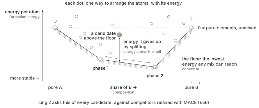
Ong, Wang, Kang and Ceder built phase diagrams this way from first-principles energies in 2008, and materials databases now report stability the same way. With more than two elements the string becomes a sheet, and finding the cheapest mixture under a composition is a small linear program: non-negative amounts of the known phases that add up to the right composition at the lowest total energy.
Temperature tilts the comparison
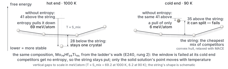
A random solid solution has something a compound lacks: many ways to arrange its atoms. That configurational entropy lowers its free energy by \(T\,S_{\text{mix}}\), with \(S_{\text{mix}} = -k_B\sum_i x_i \ln x_i\) for an ideal random mixture. For eight elements in equal parts the saving is about 180 meV/atom at 1000 K but only 16 meV/atom at 90 K (E56). So a solid solution that is stable at the hot end of the service window can be unstable at the cold end. For this project the cold end decides.
The ladder's measure is the driving force
the gap between the solid solution's free energy and the cheapest mixture of competitors, evaluated at 90 K and at 1000 K. A positive \(d\) means something off the lattice is lower. The bookkeeping is deliberately one-sided: the solid solution gets its ideal entropy, the competitors get none, and a split into two solid solutions, which would keep some entropy, is scored as less favourable than it really is. So \(d\) is a lower bound, and a composition the rung calls unstable is unstable.
The competitor the lattice cannot hold
In the refractory metals the commonest competitor is a Laves phase. It is a compound of formula AB₂ in which a large atom and a small atom pack more tightly than either could on a bcc lattice. The cubic form is named after MgCu₂ (C15) and the hexagonal ones after MgZn₂ (C14) and MgNi₂ (C36); they differ only in how the same layers are stacked. Laves phases are the largest group of intermetallic compounds (Stein, Palm and Sauthoff 2004).
No assignment of atoms to bcc sites produces a Laves phase. A cluster expansion fitted on bcc arrangements therefore cannot represent one at all: not as a competitor, not as an instability, not as a warning.
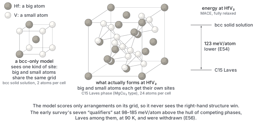
This is not a small correction. At the same composition, the C15 phases HfV₂ and ZrV₂ lie 123 and 119 meV/atom below the bcc solid solution, all relaxed with the same machine-learned potential, MACE, described at the end of this chapter (E54). That gap is more than twenty times the expansion's cross-validation error at the time. It is also more than the whole ordering effect the expansion exists to measure.
What the check showed
In short, the check reversed the survey (E56). Every composition a lattice-only survey had rated best was unstable off the lattice, and the one it had rejected was stable.
The survey's seven best were all rich in V, Hf and Zr. The check relaxed 136 competitors, among them every pair of elements as a C14 and a C15 Laves phase, and measured how far each composition sat from the hull:
| composition | survey's verdict | distance from the hull |
|---|---|---|
| the seven, rich in V, Hf and Zr | best | 98 to 185 meV/atom above it at 90 K |
| equiatomic MoNbTaW | rejected | 57 meV/atom below it at 90 K, 165 below at 1000 K |
Nothing in the set beat MoNbTaW anywhere.
Two lessons were built into the ladder.
- A lattice model's confidence says nothing about whether the lattice is right. A guard based on distance from the training data cannot catch it either, because every training structure was bcc.
- The reward a generator is paid must include the off-lattice check. A search rewarded on ordering alone would learn to find Laves formers, and would be doing its job perfectly.
A potential that lets atoms move
Comparing bcc with a Laves phase needs energies of crystals whose atoms are free to relax. Density functional theory (chapter 10) takes hours per cell; an interatomic potential takes seconds. It writes the energy as a sum over atoms, each atom's share depending only on its neighbours within a few ångströms, fitted to first-principles energies and forces.
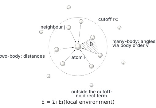
MACE (Batatia, Kovács, Simm, Ortner and Csányi 2022) builds each atom's share from messages passed between neighbours; each message already carries four-body information, so two rounds are enough. A foundation version, MACE-MP-0 (Batatia and co-authors, 2023; published 2025), was trained once on public Materials Project relaxation data and is meant to be used without refitting. This project uses its successor, MACE-MPA-0, trained on the same data plus a subsample of the Alexandria database.
It is checked where it is used. In short: it is accurate near equilibrium and much less so far from it, and against first-principles energies it is shifted by a nearly constant amount, which cancels when alloys are compared.
| check | result |
|---|---|
| 300 independent refractory structures near their equilibrium volume | error 6.61 meV/atom |
| the same, far from equilibrium | error 62 meV/atom |
| against Quantum ESPRESSO on identical cells | over-binds every alloy by 26 to 30 meV/atom |
| gaps between alloys, which are what a ranking uses | agree with Quantum ESPRESSO to 1 and 4 meV/atom |
The first two rows are E18, the last two E78.
Rung 2 as it runs
For a composition, rung 2 builds three random 54-atom bcc cells, relaxes each with MACE-MPA-0 (cell shape and atomic positions both free), and averages their energies. It compares that energy with a hull of 671 relaxed phases (E147).
Counted by size, 168 of the hull's phases are of one element and 503 of two. Counted by origin, 136 are the hand-built prototypes and 535 come from the Alexandria, Materials Cloud and JARVIS databases, fetched through their common query interface, OPTIMADE (E84; the source of each is tagged in data/offlattice_hull12.json). All were relaxed with the same potential and settings.
Only relaxed energies are ever compared with this hull. Relaxation is worth 16 to 112 meV/atom across the design space (E59), the same size as the answer. A composition costs 8 to 34 seconds, median 11, on one CPU (measured 2026-09-21, forager/ladder/spec.py).
Rung 2 can only lower a verdict. In the walk of chapter 13 it removed two compositions that the lattice rungs had passed: Mo₇₉Hf₁₉ and Mo₇₀Hf₂₀Ti₁₀. Their solid solutions sit 61 and 35 meV/atom above the cheapest off-lattice mixture at 90 K (E240).
What rung 2 cannot see
The hull holds no compound of three or more elements (E147). Where a missing ternary compound is more stable than the best binary mixture, the hull sits too high and the driving force is too optimistic: the same one-signed failure as the Laves phases above. One relaxed cell is also one arrangement, not an ensemble, and the potential knows nothing of magnetism. Those holes are listed with the rest in chapter 11.
Chapter 9
Getting there in time
Picture a full lecture hall where everyone would rather sit next to a friend. There is one empty seat in a thousand, and the only way to move is to step into an empty seat next to you. If stepping is easy the room sorts itself out within minutes. If it is hard, and the empty seats are rare, the room stays mixed up for longer than the lecture lasts.
Chapters 4 to 8 asked what an alloy would rather be: ordered or random, bcc or something else. That is the question of equilibrium. This chapter asks whether the alloy can get there within the life of a part. A free energy says what an alloy would rather be, not what it becomes.
How atoms move in a metal
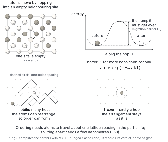
In a metal crystal an atom almost never squeezes between its neighbours or trades places with one directly. It moves by stepping into a neighbouring site that happens to be empty: a vacancy. Huntington and Seitz compared the three candidate mechanisms for copper in 1942 and found the vacancy one strongly preferred, and it has been the standard picture of diffusion in close-packed and bcc (body-centred cubic) metals since.
Two costs set how fast this goes. The first is making the vacancy. Removing an atom from the crystal costs a formation energy \(E_f\), and at temperature \(T\) only a fraction of about \(e^{-E_f/k_BT}\) of the sites are empty. The second is the hop itself. The neighbour has to squeeze through a gap between other atoms, over an energy barrier \(E_m\), the migration energy. It succeeds at a rate proportional to \(e^{-E_m/k_BT}\); Vineyard (1957) gave the prefactor in terms of the vibrations at the minimum and at the saddle point.
Multiply the two and the diffusion coefficient takes the familiar form
and the distance a typical atom travels in time \(t\) is about \(\sqrt{D\,t}\). Because \(Q\) sits in an exponent, an error of one electronvolt in it is a factor of about \(10^5\) in \(D\) at 1000 K.
How far is far enough
Different changes need different distances. Ordering on the lattice is a local shuffle: each atom needs to trade places with a neighbour or two, about 0.3 nm. Decomposing into two phases needs a species to gather into a nucleus, about 2 nm. The ladder asks, at the top of the service window and over the part's service life, whether even the most mobile atoms can travel that far (forager/ladder/rungs.py, passes_requirement).
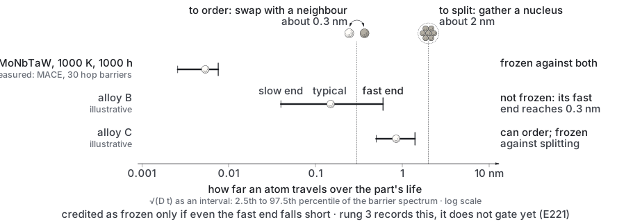
The scale of the answer can be enormous: between two alloys, a factor of five hundred million in distance. Both examples use numbers computed in this project (E58):
| alloy | activation energy \(Q\) | distance its atoms travel in a thousand hours at 1000 K |
|---|---|---|
| equiatomic MoNbTaW | 4.92 eV | 0.0025 nm, a hundredth of a lattice spacing |
| V₃₁Hf₂₉Ti₁₀W₁₀ | 1.48 eV | 1.1 mm |
The first cannot order even though its equilibrium ordering temperature lies inside the window. The second can do anything it likes. This pair is the case that put kinetics into the ladder: without it, the lattice rungs reject an alloy whose atoms cannot reach the order they would prefer.
Many barriers, and the lowest ones win
In a pure metal every hop looks the same. In a concentrated alloy every site has different neighbours, so the barriers form a broad distribution. The total hopping rate is a sum of exponentials, and a sum of exponentials is dominated by its largest terms: the easy paths carry the diffusion. The barrier that matters is therefore not the average one but a rate-weighted effective value near the bottom of the distribution.
More elements make the distribution broader, which makes the effective barrier lower and the alloy faster. This runs against the "sluggish diffusion" often assumed for high-entropy alloys, which Tsai, Tsai and Yeh (2013) measured in the face-centred cubic Co–Cr–Fe–Mn–Ni family.
Ignoring the spread makes alloys look frozen when they are not. A cheap rule that estimated \(Q\) from melting points over-predicted it, always in that direction, and by more the more elements an alloy had (E92):
| elements | the rule's over-prediction of \(Q\) |
|---|---|
| three | 0.17 eV |
| seven | about 0.7 eV |
| eight | 1.58 eV |
The eight-element alloy travels 172 nm in service, where the rule said about 0.02 nm. The rung was rebuilt to measure barriers directly.
Rung 3 as it runs
For a composition, rung 3 takes a 54-atom bcc cell and uses MACE-MPA-0, the machine-learned potential of chapter 8, for two things:
- Making vacancies. Vacancy formation energies are computed at three sites for every element above 5 per cent.
- Hopping into them. Migration barriers are computed along 30 hops, each by the climbing-image nudged elastic band method (Henkelman, Uberuaga and Jónsson 2000), which finds the saddle point of the path an atom takes into the vacancy.
Both are combined with Boltzmann weights into effective values. The travel distance is then reported as an interval, not a single number: from the 2.5th to the 97.5th percentile of a barrier spectrum fitted to the bands. It is computed at the top of the window and at the alloy's own ordering temperature. On MoNbTaW the rung costs 3094 seconds, 52 minutes, 99 per cent of it in the migration bands (forager/ladder/spec.py).
The known biases are measured, and all point the same way: toward "too frozen".
| source of bias | effect on the barrier |
|---|---|
| effective barrier taken from few bands | over-estimated by 0.29 eV at 4 bands, 0.10 eV at 30 |
| species sum left unnormalised | adds about 0.12 eV at eight elements |
At 30 bands with the sum normalised, the combined bias is under 0.15 eV. For scale, one decade of travel distance spans 0.397 eV. The gate then reads the most mobile end of the interval, so an over-estimated barrier cannot manufacture stability on its own.
Which way rung 3 can move a verdict
Kinetics can only rescue an alloy, never condemn one: a change the thermodynamics does not want does not become more likely because atoms move fast. Rung 3 therefore enters as a reachability factor \(r\) between 0 and 1,
so that as transport gets harder (\(r \to 0\)) the probability of surviving the window rises toward one, and with free transport (\(r = 1\)) the equilibrium verdict \(p\) stands. This asymmetry is what lets the ladder stop early on a confident pass at rung 2: nothing above can lower it.
Trusting the potential here
A vacancy is a defect, and a foundation potential trained mostly on perfect crystals has to be checked on defects before its numbers gate anything. On pure molybdenum it passes. The vacancy formation energy in a 16-atom cell is 3.164 eV by density functional theory (DFT, chapter 10) and 3.107 eV by MACE, a residual of −0.06 eV (E219). That says MACE's vacancy energies are not generically off, but it licenses nothing about alloys, where every site has a different neighbourhood.
The alloy anchor, the same measurement on a 16-atom MoNbTaW cell with one vacancy per element (E221), has not finished. Until it scores, rung 3 records its numbers without gating anything (trust_kinetics is off), and the search walks of chapter 13 do not climb it.
What rung 3 cannot see
It is bulk diffusion only. Grain boundaries and dislocations are short-circuit paths that can be orders of magnitude faster, and radiation or interstitial atoms open transport routes that a vacancy calculation does not contain. A real part has grain boundaries and dislocations whatever alloy it is made from.
Chapter 10
Ground truth
A kitchen scale is checked against a certified weight. The weight is not perfect either, but its error is stated, small and the same every time, so a scale that disagrees with it is the one that is wrong. In this project every cheaper rung is a scale. Density functional theory (DFT) is the certified weight they are checked against.
This chapter is about what that weight is, how it is computed, the settings that define it, and the checks that keep it honest.
Electrons as a cloud, not as a crowd
The energy of a crystal is set by its electrons. Solving for all of them at once means a wavefunction with three coordinates for every electron; for 54 refractory atoms with a dozen or more valence electrons each, there are far too many coordinates to store, let alone to search.
Hohenberg and Kohn proved in 1964 that the ground-state energy is fixed by the electron density alone, the cloud of charge in three-dimensional space, and that the true density is the one that minimises it. Kohn and Sham showed the next year how to use this. Replace the real, interacting electrons by fictitious non-interacting ones that move in an effective potential chosen so that they reproduce the same density. Non-interacting electrons are easy: each obeys its own one-particle equation,
The catch is that the effective potential depends on the density, and the density depends on the orbitals the potential produces. So the equations are solved in a loop: guess a density, build the potential, solve for the orbitals, build a new density, mix it with the old one, and repeat until nothing changes. A converged loop is called self-consistent.
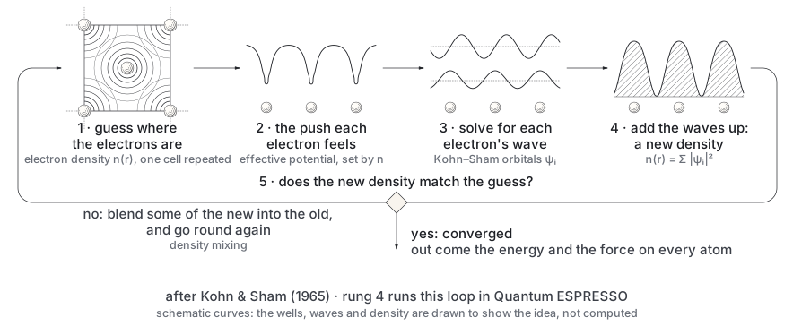
Everything the non-interacting picture leaves out is collected in one term, the exchange–correlation potential. The theory is exact if that term is exact; in practice it is approximated. This project uses the generalised-gradient form of Perdew, Burke and Ernzerhof (PBE, 1996), the same functional the training data and the screening potential were computed with, so every rung shares one reference.
The settings that define the weight
A calculation is only reproducible if its numerical choices are fixed. The ladder's rung-4 standard is (E242):
- Code: Quantum ESPRESSO (Giannozzi et al. 2009, 2017), plane waves.
- Core electrons: projector-augmented-wave datasets (Blöchl 1994) from Dal Corso's PSlibrary 1.0.0, with the semicore states of each metal treated as valence.
- Basis: wavefunction cutoff 60 Ry, density cutoff 720 Ry.
- Brillouin zone: a 4×4×4 Monkhorst–Pack mesh of sample points (Monkhorst and Pack 1976) for the 54-atom cell.
- Occupations: Marzari–Vanderbilt cold smearing (Marzari et al. 1999), width 0.02 Ry.
- Spin: not polarised, deliberately, because the labels the rung-0 model is trained on were computed that way and a spin-polarised rung 4 would not be comparable with it.
- Geometry: atoms on ideal bcc (body-centred cubic) sites at the composition's Vegard lattice constant, not relaxed.
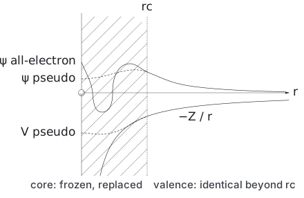
Each choice was tested where it matters. Two tests show what is at stake.
The k-point mesh, the grid on which the electrons' waves are sampled. On a 16-atom cell the answer stops changing at 6×6×6; coarser meshes are off (E87):
| mesh on the 16-atom cell | difference from the converged answer |
|---|---|
| 8×8×8 against 6×6×6 | agree to 0.17 meV/atom |
| 3×3×3 | 3.8 meV/atom |
| 2×2×2 | 56 meV/atom off, refused outright |
The 4×4×4 mesh on the 54-atom cell, three bcc cubes on an edge, has the same k-point density as 6×6×6 on the 16-atom cell, two cubes on an edge: the converged one.
The lattice constant is part of the answer (E211). The same B2 Mo–Ta crystal was run at the lattice the cluster-expansion software uses for its mapping, which is 1.46 per cent too large; it came out 41 meV/atom off. Three independent cells at the right constant, one of 16 atoms and two of 54, agree to 0.01 meV/atom. The store of DFT results now refuses a cell whose lattice constant differs from the stated convention without saying so.
What one calculation is
A converged run gives the PBE energy of one arrangement of atoms, in one cell, at one set of numerical parameters, at zero temperature. It says nothing on its own about whether the cell is large enough, whether the arrangement is the one nature picks, or whether the alloy forms. Those are separate questions, each answered by comparing calculations, never by one.
On a rented graphics processor
Rung-4 cells run on a rented A100 graphics processor (GPU) using the GPU build of Quantum ESPRESSO 7.3.1. Before any result from it was used, one cell already computed locally was re-run there with an identical input: the two total energies agree to 0.025 meV/atom (EXPERIMENTS.md, "Compute moves", 2026-09-22). A 54-atom cell takes 1 h 11 min to 1 h 24 min on the GPU, against 3.4 to 4.5 hours on six local cores (the three cells of E223, wall times in runs/e223_dft_cells/*/pw.out).
What rung 4 checks
Rung 4 does not recompute a verdict; an ordering temperature or a full hull in DFT would need thousands of calculations. It checks the numbers the verdicts rest on, in two ways.
Formation energies. For the three random cells the first search sent up the ladder, DFT and the rung-0 model then in use compare directly (E223):
| cell | DFT (meV/atom) | rung-0 model then in use (meV/atom) |
|---|---|---|
| first | −56.5 | −56.9 |
| second | −31.2 | −29.6 |
| third | −14.3 | −29.8 |
The model that now ships is off by 0.4 to 13.5 meV/atom on the same cells, 6.1 on average (E237).
Ordering energies. Here rung 4 compares a model's own ground state with a random arrangement at the same composition. On Cr₂₅Ta₂₅Ti₂₅W₂₅ the earlier model said 107.9 meV/atom; DFT puts the ordering energy at 44.9 — the right pair, the wrong size (E222).
Every such cell enters the store and becomes a known answer for the next model.
Pinning the references
The rung-0 labels are formation energies, and a formation energy subtracts one pure-element reference per element. For titanium, chromium and hafnium the public data pin those references poorly. Titanium has three pure-element structures ("frames") in the data; hafnium has twelve, spread over 34 meV/atom. Two defensible ways of picking the reference differ by 33.5, 28.1 and 22.0 meV/atom per unit fraction of Ti, Cr and Hf respectively (E239).
In short: ordering is safe, absolute energies are not. The error this leaves is linear in composition, so it cancels exactly in any energy difference at fixed composition. Ordering and the transition temperature (rung 1) are untouched. Absolute formation energies move, and with them the rung-0 screen and the hull comparison.
The fix is to measure the error. About 48 of the dataset's own ordered cells are recomputed at the rung-4 standard, chosen before any DFT so that every element and every Ti, Cr and Hf pairing is covered. The differences are fitted as
one reference shift \(\delta\mu_i\) per element, with bootstrap intervals. Any shift more than two standard errors from zero is applied to the labels. The rung-0 model is then refitted and re-scored on cells it never saw. At the time of writing the anchor cells are running.
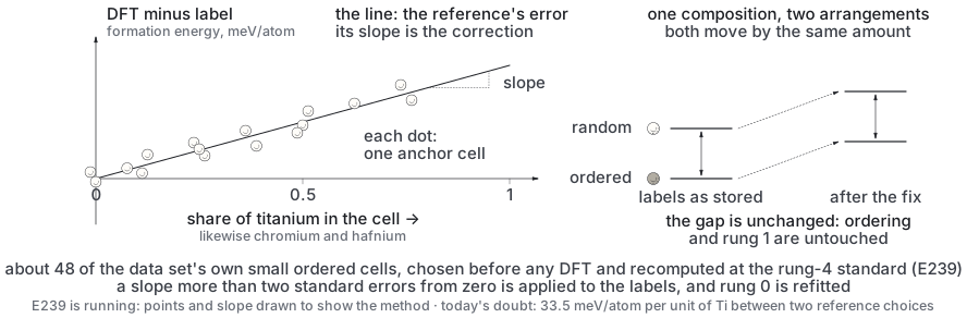
Spin, and a loop that would not settle
The refractory rung is non-magnetic by design. But the ladder also carries a spin-polarised branch for cells containing iron, cobalt, nickel or chromium, where ignoring magnetism is not a small error. At each element's own minimum, spin lowers the energy by about 12 meV/atom for Cr, 61 for Ni, 170 for Co and 460 for Fe (E216).
Spin makes the self-consistent loop harder. In one test the magnetism settled quickly but the charge never did (E225). On a 16-atom ordered Ni₁₂Fe₄ cell the total magnetic moment settled at 19.4 μB (Bohr magnetons) within twenty steps. The loop's error then swung across three orders of magnitude, from hundredths of a rydberg to tens of rydbergs, for 180 more steps without converging (0.031 to 33.6 Ry in the kept first attempt, pw.out.attempt1). That is charge sloshing back and forth, not a search for the magnetic state. The standard retry, lowering the mixing fraction, cannot cure it.
The spin-aware ladder does two stages:
- Converge the cell with wider smearing (2.5 times the production width), plain mixing, and starting moments rescaled to what the failed run found.
- Restart at the production settings from that density.
Cutoffs, smearing, k-mesh and convergence threshold of the production run never change, and only the production energy is accepted. On the same Ni₁₂Fe₄ cell both stages converged: the first in 89 iterations, the production restart in 17. The total moment was 19.39 μB per cell, the moment the failing run had settled at (runs/scf_spin_test/Ni12Fe4_ordered_nspin2.log). The survivor's cells in chapter 13 go through this ladder.
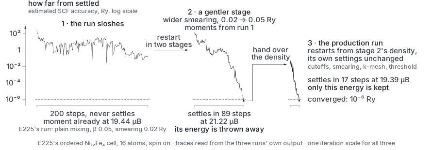
What rung 4 cannot see
It is static: no vibrations, no temperature. It is one arrangement per cell, so it has no configurational entropy of its own. Its refractory branch is non-magnetic on purpose, so chromium's reference is non-magnetic bcc Cr, which is not the ground state of real chromium. And it is only as good as PBE, which for transition metals is good but not exact.
Chapter 11
The fidelity ladder
A doctor does not order a biopsy for every patient. A questionnaire comes first, then a blood test, then a scan, and only the few whom every earlier step could not clear go further. Each step costs more and asks a sharper question. Most patients stop early, and nobody is declared healthy because the cheapest test liked them.
The ladder is that procedure for alloys. Chapters 5 to 10 described its rungs one at a time; this chapter puts them together, says what each costs, how a verdict moves from one to the next, and how the ladder is kept honest.
One question, five prices
Every rung answers the same question — the probability that a composition keeps one bcc (body-centred cubic) solid solution with no phase change anywhere from 90 to 1000 K — so that a promotion is a decision and a disagreement is a lesson. What changes from rung to rung is not only the precision but the physics: each rung adds something the one below cannot see. That is what distinguishes a fidelity ladder from running the same model longer.
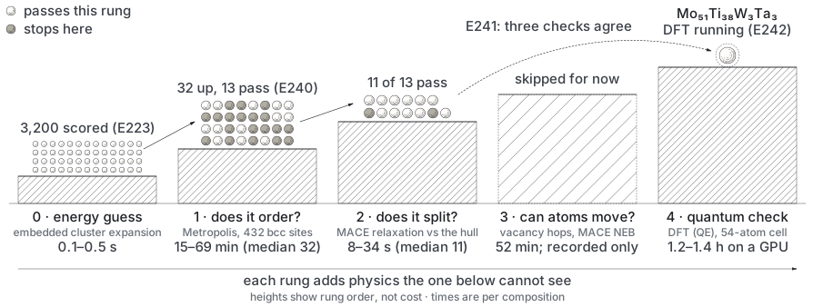
What each rung asks, costs and was checked against (DFT is density functional theory, the top rung):
| rung | asks | cost per composition | checked against |
|---|---|---|---|
| 0 · screen | the random solid solution's formation energy, and how far below the off-lattice hull | 0.1–0.5 s | 7.5 meV/atom mean error on eleven independent DFT cells; 6.1 on the search's own random cells (E237) |
| 1 · ordering | does it order on the lattice inside the window? | about half an hour (E240) | equiatomic Mo–Ta, below |
| 2 · off-lattice | is bcc the right lattice at all? | 8–34 s | gaps agree with DFT to 1 and 4 meV/atom (E78) |
| 3 · kinetics | can the atoms get there within the service life? | 52 min | pure Mo vacancy, 3.107 vs 3.164 eV (E219) |
| 4 · first principles | do the energies the verdicts rest on hold? | 1.2–1.4 h per 54-atom cell on a rented A100 graphics processor (GPU) | three B2 Mo–Ta cells agree to 0.01 meV/atom (E211) |
From the bottom rung to the top the price rises by four orders of magnitude. That is why most compositions must stop low.
Costs are measured, not assumed, and recorded with their source in forager/ladder/spec.py. The rung-1 figure is the wall time of a walk up rungs 0 to 2: 15 to 69 minutes per composition, median 32 (E240, runs/e240_rescored/summary.jsonl).
How a verdict moves
Rung 1 asks whether the alloy orders anywhere inside the window. It turns an ordering temperature into a probability that the transition lies outside the window, with the temperature grid's step as its resolution.
It cools a 432-site cell from 2600 K down to 60 K, below the window's floor. The heat capacity is read two ways: from the slope of energy against temperature, and from the energy's fluctuations. In equilibrium they are the same quantity. The two readings decide the verdict (E240):
| the two readings | verdict |
|---|---|
| a peak inside the window, in either reading | fails |
| both silent down to 60 K | passes the floor; scored as a transition bounded below the window |
| no readable answer | no verdict, which is scored as zero, never as a number |
Rung 2 can only lower that probability: it adds the off-lattice driving force that rung 1 does not have. Rung 3 can only raise it, through the reachability factor of chapter 9, \(p' = 1 - (1-p)\,r\). The asymmetry decides where the ladder may stop early. A confident pass at rung 2 is safe, because nothing above it can take the pass away. A failure at rung 1 is not final, because kinetics may still rescue it.
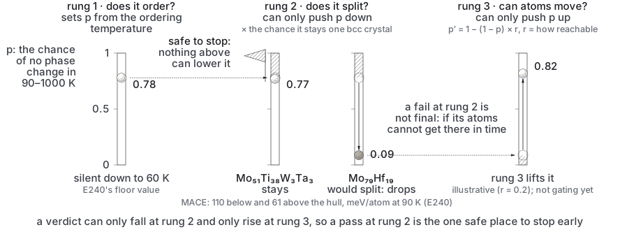
Written down before it runs
Every change to a rung is written in the experiment log as a prediction with a numerical bar before the run starts, together with what will be done for each outcome. Three examples show the pattern.
Choosing the rung-0 model (E237). The smallest embedding had to clear three bars:
| bar | limit |
|---|---|
| mean error on eleven DFT cells | 14 meV/atom or less |
| mean error on four Mo–Ta cells | below +15 |
| held-out error | 9 or less |
Embedding 5 met all three. A requirement recorded before the numbers existed — hold the search's own random cells too — removed it, and embedding 6 was chosen. The refit on corrected labels then failed its random-cell bar, 19.6 meV/atom against 8 (E238). So the fallback written in advance shipped: the embedding-6 model on the old labels remains rung 0 and rung 1.
Testing the survivor at DFT (E242). An ordering energy of 5 meV/atom or less confirms the model at that composition; 5 to 15 is not established; above 15 the find fails.
Testing the generator (E224, chapter 12). The real wiring must beat its rewired copy on all five seeds, by a median of at least 31 finds.
A failed bar is reported as failed, with the number. And because one fit hides how uncertain a rung's model is, every rung-0 model is a three-seed ensemble, with its seed spread reported beside its error.
Known answers
A rung is trusted only after it reproduces something already known, run through the same code the ladder uses.
The sampler's temperature. The package's own sampler runs at twice its nominal temperature. The test was a cluster expansion built to be exactly a nearest-neighbour Ising model (the textbook model of ordering on a lattice), sampled both by the package and by an independent sampler. Measured on a fine grid, the factor is 2.000 ± 0.03 (E215c). The ladder reports physical temperatures.
The fast evaluator. Rung 1 evaluates the model through an exact re-implementation of its forward pass, the calculation that turns an arrangement of atoms into an energy. It gives the same numbers: on the production cell it agrees with the package's own evaluation to within 6.3 × 10⁻⁷ eV per cell and 0.023 meV per swap. It is much faster: at the largest embedding tested it runs 1,519 swap evaluations per second against 28, a factor of 54 (the exact-evaluator record under E237).
Mo–Ta. Rung 1 finds the right order for equiatomic Mo–Ta inside the range set in advance, but not the published temperature. Through the production path it orders at 1149 ± 114 K into perfect B2, the order in which every nearest neighbour is of the other kind (Warren–Cowley \(\alpha_1 = -1.00\)). That is inside the pre-registered range of 500 to 2600 K (E242).
| Mo–Ta ordering temperature | how it was obtained | |
|---|---|---|
| this project, shipped model | 1149 ± 114 K | heat-capacity reading of a 432-site cell |
| this project, earlier rung-0 model | 985 K | the same sampler |
| published (Kim and Widom 2023) | 2020 K, carrying ±545 K by this project's own rule for a model with their stated error | a single four-site cluster model sampled by replica-exchange Monte Carlo; the susceptibility peak of a 1024-atom lattice without relaxation |
The two are not the same observable. The pass says the rung finds the right order inside the pre-registered range. It does not say the two numbers agree, and they do not: ours is 0.57 of theirs.
Published transition temperatures. Six of six comparable published systems fell within 22 per cent of the published value, with the earlier model and the corrected sampler (Sobieraj et al. 2020; Fernández-Caballero et al. 2017). The seventh, Cr–Ta–Ti–W, came out at 2.92 times the published value; DFT traced that to one overstated pair (E222).
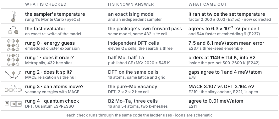
Machine-checked conventions
The conventions themselves. Six identities the ladder's numbers rest on are proved in Lean 4, a proof assistant, with its mathematics library Mathlib (formal/). Each is tied to a test of the production function that computes it. The six:
- the factor-of-two temperature convention;
- detailed balance and stationarity of the swap move;
- the decoding of the package's short-range-order output: exact when the order parameter is negative, and provably impossible when it is not;
- the symmetry of the Warren–Cowley parameter and its lower bound \(\max(1 - 1/x_a,\,1 - 1/x_b)\), reached only by perfect order;
- that a label computed inside its volume bracket can only be raised by a missed minimum;
- the algebra of the fast evaluator.
The statements and their ties to the code were then tested. An adversarial review of the statements found two overclaims, both fixed. Four deliberate code mutations were made, and every one was caught. No proof found the code disagreeing with the mathematics (the formal-checks record under E238).
What the ladder cannot see
- Magnetism. The ladder is spin-blind in its refractory branch. So three changes inside the window are invisible to it: the Néel transition of chromium (311 K) and the Curie transition of nickel (627 K), where each orders magnetically, and cobalt's structural change (695 K) (
forager/ladder/spec.py). - Compounds of three or more elements. The off-lattice hull holds none.
- Large ordered patterns. Rung 1's 432-site cell cannot hold every ordered superstructure. Mo–Ta's true ground state is B2 with periodic antiphase faults, 1 meV/atom below B2, which no cubic cell used here admits.
- Kinetics beyond the bulk. Rung 3 is bulk diffusion only, and does not yet gate.
And the ladder answers feasibility, nothing else. Oxidation, density, cold brittleness and liquid-oxygen compatibility are applied afterwards, by a separate selection layer that trades them against each other (forager/evaluate/selection.py). Folding them into the ladder's number would hide a trade-off behind a score.
Chapter 12
The generator
A search party is looking for the lowest valleys in fog. No one can see the landscape; each walker can only tell whether the ground under their feet is better or worse than a moment ago. So each keeps walking while things improve and turns in a random new direction when they get worse. Bacteria find food exactly this way, running straight and tumbling at random, as Berg and Brown showed by tracking single E. coli in 1972. What tells the walkers "better" is a guide who gives every spot a score, and who revises the scores as reports come back of what each valley actually held.
The generator is that search party on the space of compositions. The walkers are points on the simplex of nine element fractions; the guide is a network wired as a fly's brain; the reports are verdicts from the ladder.
Why a generator, not a chooser
A chooser scores a fixed list of candidates, so the list is its ceiling. A generator has no list: it proposes compositions, is told what the ladder made of them, and proposes again. Every search arm in the project, from a uniform random draw to the fly, answers the same two calls, propose and observe, under the same budget. That interchangeability is the experiment: a learning arm has to beat itself with learning switched off, and the simple baselines, or its learning is decoration.
The wiring of a whole fly's brain
The guide's wiring is the MaleCNS connectome, the complete central nervous system (CNS) of one adult male Drosophila melanogaster, reconstructed from electron microscopy at 8 nm resolution, proofread and annotated by the FlyEM team at the Howard Hughes Medical Institute's Janelia campus (HHMI Janelia) with the University of Cambridge, the Medical Research Council (MRC) Laboratory of Molecular Biology and Google Research: about 166,700 neurons in the brain and nerve cord (Berg et al. 2026). The project's copy of it has 164,506 neurons and 25,135,527 directed connections (E152), each connection weighted by its synapse count and signed by the predicted transmitter of the neuron it leaves: γ-aminobutyric acid (GABA), glutamate and histamine inhibit.
Neuron shapes, timing, spikes and synaptic chemistry are discarded. This is not a simulation of a fly but a recurrent network whose wiring happens to be a fly's, and whether that wiring helps has to be measured.
The mushroom body
The part of the fly's brain that learns what an odour is worth is the mushroom body, mapped by Aso and colleagues in 2014; its logic is the template for how the guide learns. Odours arrive through about fifty channels and are spread onto some 2,000 Kenyon cells per hemisphere, each of which fires only for a particular combination, so any one odour lights up a small, distinctive set. The Kenyon cells' long axons are read by 21 types of output neuron, whose dendrites tile the lobes into 15 compartments. Each of 20 types of dopamine neuron sends its axons into one or two of those compartments and reports reward or punishment there.
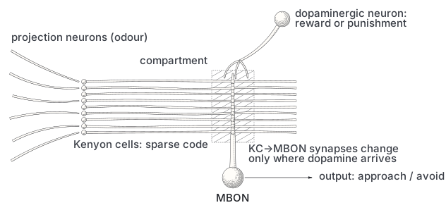
Learning happens at one place, the synapse from a Kenyon cell onto an output neuron, and needs three factors at once. In the project's copy of the brain the circuit has:
| part of the circuit | count |
|---|---|
| Kenyon cells | 4,064 |
| output neurons | 97 |
| dopamine neurons of the PAM (protocerebral anterior medial) cluster | 316 |
| dopamine neurons of the PPL1 (protocerebral posterior lateral 1) cluster | 24 |
| APL (anterior paired lateral) inhibitory neurons | two |
| olfactory projection neurons | 595 |
| Kenyon-cell-to-output synapses that can learn | 61,210 |
The synapse count is from E152, the rest from E7.
From a composition to a score
A composition enters the network as a sensory stimulus and leaves it as one score, in three steps:
- In. Its nine fractions are projected by a fixed random map onto all 17,479 sensory neurons of the connectome (E163).
- Through. Activity spreads for four steps through the whole measured wiring.
- Out. The score is read from 794 neurons on the output side — the 97 mushroom-body output neurons, 665 neurons of the lateral accessory lobe and 32 descending neurons of the DNa group — weighted by a readout that is learned rather than assumed (E159). Reading fixed dynamics through a trained linear layer is the reservoir construction used for fly connectomes by Morra and Daley (2023) and Costi et al. (2025).
The Kenyon-cell layer is kept sparse, as in the fly, by a threshold calibrated on the codes that the swarm's own proposals evoke. Calibrating it on anything else starved the code. At one point three of the 4,064 cells were active, and nothing could be learned until the calibration was moved (E61).
How the guide learns
Each composition the swarm proposes goes to the ladder's screen, which returns a driving force \(d\) in meV/atom at 90 K. It becomes a probability \(p = 1/(1 + e^{d/25})\) and a reward \(r = 2p - 1\) between −1 and +1. The learning signal is a prediction error: how much better the reward was than the guide's own score for that composition expected, each measured against its running average and spread,
The same \(\delta\) updates the readout weights and the Kenyon-cell-to-output synapses, each in proportion to its own input activity. Bennett, Philippides and Nowotny (2021) proposed that the fly's dopamine neurons carry such a prediction error to the mushroom body; here it is one number broadcast to every learning synapse.
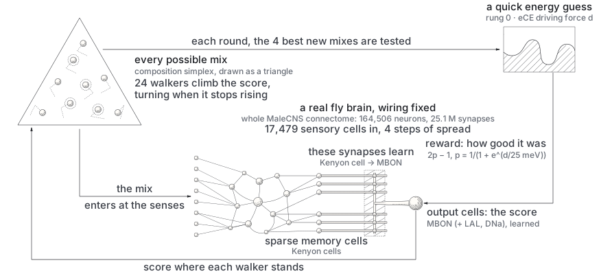
The swarm
The swarm's rules:
- Moving. Twenty-four walkers run and tumble on the simplex with a step of 0.05, keeping their heading while the score improves and turning when it does not. A walker that stalls is restarted at a random composition.
- Proposing. Each round the four best-scored positions go to the ladder, provided they are not within 0.05 (in summed fraction differences) of anything proposed before. A run is 200 rounds, 800 compositions.
- Counting. A composition counts as a find when its driving force is below −40 meV/atom at 90 K. Finds count as distinct when they differ by at least 0.15.
Each walker's step length and patience are fixed at random. The brain's own attempt to set them made the search worse: the worst of three versions on two different rewards (E198b).
What the controls show
Against its frozen twin. The readout learns the reward. The twin has the same wiring, walkers and budget, with learning switched off (E201):
| learning | frozen | |
|---|---|---|
| how well its score ranks the ladder's reward (Spearman correlation) | +0.90 | −0.03 |
| distinct finds | 181.5 | 26 |
Against keep-the-best-and-mutate. The fly finds wider, not better. On the same reward it makes more distinct finds than the elitist hill-climber, at the same rate, and its finds are shallower (E195c, E201b):
| fly | elitist hill-climber | |
|---|---|---|
| distinct finds, three seeds | 299 ± 31 | 238 ± 14 |
| rate at which finds accumulate | 147 | 145 |
| depth of finds, two seeds (meV/atom) | −66.8 | −73.7 |
The fly's lead is 61 finds, about two seed standard deviations; the rate is a tie. The fly also carries three devices for spreading out that the elitist lacks — the novelty filter, restarts on stall and three times as many walkers — and its hit rate equals the elitist's (the adversarial review recorded in the log before E224).
The rewiring test
Against its own wiring, rewired. This is the decisive test, E224. It asks whether the fly's particular wiring matters, or whether a rewired copy would do as well. It pairs, seed by seed:
- A, the real wiring;
- B, a copy with every connection rewired while each neuron keeps its number of inputs and outputs;
- C, a random head matched in sparsity;
- D, the frozen twin;
- four arms without a brain: elitist, elitist with the fly's three devices, a linear ridge readout driving the same swarm, and MAP-Elites (Multi-dimensional Archive of Phenotypic Elites, a search that keeps the best find in each of many niches).
Its bar, written before it ran: A beats B on all five seeds, by a median of at least 31 distinct finds.
The bar is not met. The real wiring beats its rewired copy on two seeds and loses on three:
| seed | real wiring (A) | rewired (B) | random head (C) | A minus B |
|---|---|---|---|---|
| 0 | 333 | 301 | 290 | +32 |
| 1 | 278 | 332 | 245 | −54 |
| 2 | 333 | 315 | 319 | +18 |
| 3 | 15 | 240 | 1 | −225 |
| 4 | 203 | 334 | 330 | −131 |
Distinct finds per seed, 800 verifications each (runs/e224_{A,B,C}_s*.log). The signs disagree and the median of A minus B is −54.
Seed 3 needs a note. There the real and random heads found almost nothing for 150 rounds, while the rewired head started at once: the real wiring made 0, 0, 1 and 34 finds per 50-round window. A replay of that seed with a full decision ledger is queued.
The frozen twin (D) and the four brainless arms were still running when this was written, so the experiment as a whole is not yet scored.
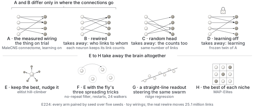
The field's recent work points the same way. A degree-preserving rewired null removed an apparent connectome advantage in a flyvis model (Dhiman 2026), and a whole-connectome reservoir's reproducible benefit was resistance to overfitting, not accuracy (Costi et al. 2025).
What this means
The generator is a working searcher: its readout learns the ladder's reward, it beats its own frozen twin by a wide margin, and it finds more distinct alloys than a hill-climber at the same rate. No measurement so far attributes that to the fly's particular wiring rather than to properties a rewired copy shares with it.
Chapter 13
What the ladder found
Pour gravel through a stack of sieves, coarse on top and fine at the bottom, and weigh what is left on each. Most of the gravel stops in the first sieves; what reaches the bottom is small and has passed every test above it. This chapter is that weighing for the first search run on the corrected ladder: what went in, where each composition stopped, the one that was chosen for the last and most expensive test, and what is still open.
What went in
The input was 32 compositions: the leading finds of the first search to climb the corrected ladder (E223). That search ran two generators, the fly and the elitist hill-climber, on two seeds each over the nine elements. Each run was 200 rounds of four proposals, paid by the rung-0 screen alone. The leaders of its finds were pooled, de-duplicated by composition and capped at 32: 18 from the fly and 14 from the hill-climber. They were walked up the ladder one at a time, each result on disk before the next began.
They were then walked again on the model that ships (E240): the embedding-6 cluster expansion of chapter 6, the mean of three seeds, evaluated exactly at rung 1 (chapter 7). Each composition was cooled on a 432-site cell from 2600 K down to 60 K, below the window's 90 K floor. It was read both ways drawn in chapter 7 and described in chapter 11: from the slope of energy against temperature, and from the energy's fluctuations. Both can show spurious peaks at the cold end, where the sampler freezes. So the slope reading is read first, and the fluctuation reading is consulted when the slope's maximum sits at the floor.
Rung 3 was not climbed, because it does not yet gate (chapter 9).
Where they stopped
Eleven of the 32 pass rungs 0 to 2. All 24 finds that the first walk had left without a verdict now carry one, and 18 of the 32 verdicts changed (E240).
| step | compositions |
|---|---|
| walked | 32 |
| no transition in either reading down to 60 K | 13 |
| removed by rung 2 | 2 |
| pass rungs 0 to 2 | 11 |
Rung 2 removed Mo₇₉Hf₁₉ and Mo₇₀Hf₂₀Ti₁₀: their solid solutions sit 61 and 35 meV/atom above the cheapest mixture of off-lattice competitors at 90 K. The eleven that pass have probabilities of surviving the window between 0.50 and 0.77.
Five more finds were ambiguous. Their slope reading peaked only at the 60 K floor, while their fluctuation reading peaked inside the window, at 331 to 575 K. They fail. Failing an ambiguous case is the safe direction, but it does not prove those five order; they are recorded as not established (E242).
The eleven that passed
Every one of the eleven is molybdenum-rich, with titanium, niobium or tungsten as the main partner. How to read the table:
- Labels are the project's rounded names for each composition and list only the main elements; the survivor's full composition is given below.
- p is the probability of no phase change in the window after rungs 0 to 2.
- The MACE driving force is rung 2's number, from the machine-learned potential of chapter 8: negative means the solid solution lies below the cheapest off-lattice mixture.
- δ is the size mismatch and VEC the valence electron concentration; with the votes, they are explained in the next section.
| composition | p | MACE driving force at 90 K (meV/atom) | size mismatch δ | VEC | votes |
|---|---|---|---|---|---|
| Mo₅₁Ti₃₈W₃Ta₃ | 0.771 | −110.0 | 3.5 % | 5.13 | 3 |
| Mo₅₃Ti₃₃W₁₄ | 0.758 | −93.3 | 2.7 % | 5.33 | 3 |
| Mo₅₆Ti₄₁ | 0.746 | −84.1 | 3.1 % | 5.16 | 3 |
| Mo₅₈Ti₄₂ | 0.743 | −82.7 | 2.8 % | 5.16 | 3 |
| Mo₆₅W₁₆Cr₇Ti₆Nb₄ | 0.734 | −77.3 | 2.9 % | 5.82 | 3 |
| Mo₆₂Nb₂₃W₁₃ | 0.729 | −74.7 | 2.4 % | 5.75 | 3 |
| Mo₆₆Nb₂₂W₁₁ | 0.714 | −68.1 | 2.1 % | 5.77 | 3 |
| Mo₆₇Nb₁₂Ta₁₀Cr₆W₅ | 0.714 | −68.0 | 3.1 % | 5.77 | 3 |
| Mo₆₉W₂₅Nb₆ | 0.642 | −45.9 | 1.3 % | 5.94 | 3 |
| Mo₅₈Ti₃₄Hf₈ | 0.503 | −18.3 | 3.9 % | 5.16 | 3 |
| Mo₅₉Ti₃₀W₁₁ | 0.774 | −115.4 | 2.6 % | 5.40 | 2 |
Source: runs/e241_agreement.json (E241).
Choosing one by agreement
Density functional theory (DFT), the top rung, costs hours per cell, so one composition goes first. It was chosen by a rule written before the walk finished (E241): prefer the composition that independent models agree on, rather than the one a single learned model likes best, because a learned model is most confidently wrong exactly where it extrapolates. The rule follows Blalock and co-authors (2026), who integrated complementary sources of information for multi-objective enzyme engineering.
Three independent votes were counted for each of the eleven:
| vote | yes if | independent because |
|---|---|---|
| MACE | the relaxed solid solution sits below the cheapest off-lattice mixture | a different kind of model, trained on different data |
| two empirical rules | the atomic size mismatch \(\delta\) is below 6.6 per cent, and VEC is below 6.87 | tabulated element data |
| the earlier rung-0 model | it found no transition inside the window | fitted to different labels |
The two thresholds are published. 6.6 per cent is the bound Yang and Zhang (2012) found for high-entropy solid solutions; 6.87 is the value below which Guo and co-authors (2011) found bcc (body-centred cubic) to be the stable solid solution.
The rule — most votes, then highest probability — picked Mo₅₁Ti₃₈W₃Ta₃: probability 0.771, MACE driving force −110.0 meV/atom, size mismatch 3.5 per cent, valence electron concentration 5.13, and no transition in the window under either model.
Ten of the eleven earned all three votes. The one with the highest probability, Mo₅₉Ti₃₀W₁₁, lost the third: the earlier model found a transition in the window for it.
In full the survivor is 50.7 per cent molybdenum, 38.3 titanium, 3.2 tungsten, 3.0 tantalum and 2.2 zirconium, with 0.6 per cent each of chromium, hafnium, niobium and vanadium (runs/e242_x9.json).
The test at the top rung
E242 asks whether the survivor orders, using DFT. It compares two cells:
- Ordered. The rung-0 model anneals a 54-atom cell of the survivor's composition to the lowest-energy arrangement it can find, from five starts.
- Random. A random arrangement of the same atoms is written beside it.
Both go to Quantum ESPRESSO at the rung-4 standard of chapter 10, on ideal bcc sites at the Vegard lattice constant (3.2351 Å, runs/e242_random.log), through the spin-aware retry ladder on the rented graphics processor (GPU). The ordering energy is the difference,
per atom. The bars were written before the run:
| ordering energy | what it means |
|---|---|
| 5 meV/atom or less | the model's ordering energetics are confirmed at this composition, and the find stands as the ladder's first full pass |
| between 5 and 15 | the question is not settled: a transition could sit somewhere around 100 to 400 K, at the 20 to 30 K per meV/atom that a mean-field scaling of E222 suggests |
| above 15 | the model is wrong here and the find fails |
A small value is a lower bound, because the ordered cell is the lowest state the model finds, not necessarily the one DFT would prefer; that is stated with the result, not after it.
The result is pending. At the time of writing the model's anneal was running and the two DFT cells had not started. The same experiment first checked the model's rung 1 on a known answer: equiatomic Mo–Ta orders at 1149 ± 114 K into perfect B2, inside its pre-registered range (chapter 11). That check passed.
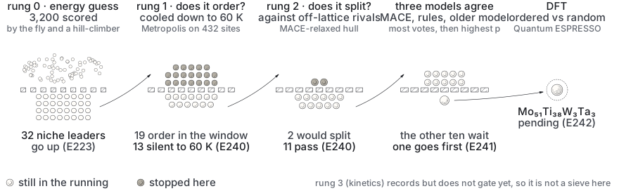
What is still open
The DFT answer. Everything above is the ladder's prediction; E242 is the first test of a search find at the top rung.
The absolute energies. The references that pin titanium's, chromium's and hafnium's formation energies are being measured by the anchor cells of E239. With 38 per cent titanium, the survivor's absolute formation energy may carry an error of the order of ten meV/atom from the titanium reference alone. The ordering question does not: the error is linear in composition and cancels in \(\Delta E_{\text{order}}\).
The kinetics. Rung 3 records but does not gate until its alloy anchor, E221, scores. None of the eleven has been credited or penalised for how fast its atoms move.
What the model and the hull cannot hold. The 432-site cell cannot hold every ordered superstructure, and the hull contains no compound of three or more elements, so a ternary competitor to Mo–Ti–W would be invisible (chapter 8). The five finds that fail on the fluctuation reading are not established either way.
Everything that is not the phase question. The ladder answers feasibility only. The selection layer that trades oxidation, density, brittleness at 90 K and compatibility with liquid oxygen has not been applied to the survivor; it treats titanium, 38 per cent of the survivor, as excluded from liquid-oxygen service (forager/evaluate/selection.py).
The generator. Eight of the eleven came from the fly and three, the survivor among them, from the hill-climber. The 32 were not balanced between the two arms, so the split says nothing about which searches better. Whether the fly's wiring contributes anything beyond what a rewired copy of it would do is E224's question, and it is not yet scored (chapter 12).
The material. No alloy has been made. Every statement in this book is about models and calculations, checked against each other and against published calculations. The first measurement on a real sample would be the next rung, and it is not part of this project.
Chapter 14
Notes and sources
Where the numbers come from
Every number in this book comes from a file in the project's repository. Most are recorded in EXPERIMENTS.md, the project's dated experiment log, and are cited by their experiment id (E56, E240, …); each id links to its page on this site, which carries the prediction written before the run, the result, and any later correction. A few numbers are read directly from run outputs and are cited by path (runs/…). What each rung asks, costs and cannot see is recorded, with the source of every figure, in forager/ladder/spec.py. The machine-checked statements of chapter 11 are in formal/, each tied to a test of the code that computes it.
Where a result was later corrected or withdrawn, the book states the current reading and the Logbook tells the history.
The references below were checked against their publishers' or preprint servers' records. Within each group the paper that originated an idea comes first.
Alloys and order on a lattice (chapters 1–7)
- J.-W. Yeh, S.-K. Chen, S.-J. Lin, J.-Y. Gan, T.-S. Chin, T.-T. Shun, C.-H. Tsau and S.-Y. Chang, "Nanostructured high-entropy alloys with multiple principal elements: novel alloy design concepts and outcomes", Advanced Engineering Materials 6, 299 (2004). doi:10.1002/adem.200300567
- B. Cantor, I. T. H. Chang, P. Knight and A. J. B. Vincent, "Microstructural development in equiatomic multicomponent alloys", Materials Science and Engineering A 375–377, 213 (2004). doi:10.1016/j.msea.2003.10.257
- O. N. Senkov, G. B. Wilks, D. B. Miracle, C. P. Chuang and P. K. Liaw, "Refractory high-entropy alloys", Intermetallics 18, 1758 (2010). doi:10.1016/j.intermet.2010.05.014
- O. N. Senkov, G. B. Wilks, J. M. Scott and D. B. Miracle, "Mechanical properties of Nb₂₅Mo₂₅Ta₂₅W₂₅ and V₂₀Nb₂₀Mo₂₀Ta₂₀W₂₀ refractory high entropy alloys", Intermetallics 19, 698 (2011). doi:10.1016/j.intermet.2011.01.004 — MoNbTaW a single disordered bcc phase after exposure to 1400 °C.
- W. L. Bragg and E. J. Williams, "The effect of thermal agitation on atomic arrangement in alloys", Proceedings of the Royal Society of London A 145, 699 (1934). doi:10.1098/rspa.1934.0132 — the order–disorder transition.
- J. M. Cowley, "An approximate theory of order in alloys", Physical Review 77, 669 (1950). doi:10.1103/PhysRev.77.669 — the short-range order parameter.
- N. Metropolis, A. W. Rosenbluth, M. N. Rosenbluth, A. H. Teller and E. Teller, "Equation of state calculations by fast computing machines", Journal of Chemical Physics 21, 1087 (1953). doi:10.1063/1.1699114
- J. M. Sanchez, F. Ducastelle and D. Gratias, "Generalized cluster description of multicomponent systems", Physica A 128, 334 (1984). doi:10.1016/0378-4371(84)90096-7 — the cluster expansion.
- Y. L. Müller and A. R. Natarajan, "Constructing multicomponent cluster expansions with machine-learning and chemical embedding", npj Computational Materials 11, 60 (2025). doi:10.1038/s41524-025-01543-3; arXiv:2409.06071 — the embedded cluster expansion.
- Y. L. Müller, C. A. Paetsch and A. R. Natarajan, "pyeCE: A Python implementation of the embedded cluster expansion", arXiv:2609.10190 (2026) — the software rungs 0 and 1 are built on.
- J. Byggmästar, "RHEA database and tabGAP/NEP potential files", Zenodo (2026). doi:10.5281/zenodo.18863415 — the DFT training labels.
Published transition temperatures (chapter 11)
- A. D. Kim and M. Widom, "Interaction models and configurational entropies of binary MoTa and the MoNbTaW high entropy alloy", Physical Review Materials 7, 063803 (2023). doi:10.1103/PhysRevMaterials.7.063803; arXiv:2212.02470 — Mo–Ta at 2020 K.
- D. Sobieraj, J. S. Wróbel, T. Rygier, K. J. Kurzydłowski, O. El Atwani, A. Devaraj, E. Martinez Saez and D. Nguyen-Manh, "Chemical short-range order in derivative Cr–Ta–Ti–V–W high entropy alloys from the first-principles thermodynamic study", Physical Chemistry Chemical Physics 22, 23929 (2020). doi:10.1039/D0CP03764H
- A. Fernández-Caballero, J. S. Wróbel, P. M. Mummery and D. Nguyen-Manh, "Short-range order in high entropy alloys: theoretical formulation and application to Mo–Nb–Ta–V–W system", Journal of Phase Equilibria and Diffusion 38, 391 (2017). doi:10.1007/s11669-017-0582-3
Leaving the lattice (chapter 8)
- S. P. Ong, L. Wang, B. Kang and G. Ceder, "Li–Fe–P–O₂ phase diagram from first principles calculations", Chemistry of Materials 20, 1798 (2008). doi:10.1021/cm702327g — the convex hull built from first-principles energies.
- F. Stein, M. Palm and G. Sauthoff, "Structure and stability of Laves phases. Part I. Critical assessment of factors controlling Laves phase stability", Intermetallics 12, 713 (2004). doi:10.1016/j.intermet.2004.02.010
- I. Batatia, D. P. Kovács, G. N. C. Simm, C. Ortner and G. Csányi, "MACE: Higher order equivariant message passing neural networks for fast and accurate force fields", Advances in Neural Information Processing Systems 35 (2022); arXiv:2206.07697
- I. Batatia et al., "A foundation model for atomistic materials chemistry", Journal of Chemical Physics 163, 184110 (2025). doi:10.1063/5.0297006; arXiv:2401.00096 — MACE-MP-0.
- MACE-MPA-0, released in the ACEsuit
mace-foundationsrepository (tagmace_mpa_0, December 2024), trained on the Materials Project trajectories plus a subsample of Alexandria; MIT licence. github.com/ACEsuit/mace-foundations - C. W. Andersen et al., "OPTIMADE, an API for exchanging materials data", Scientific Data 8, 217 (2021). doi:10.1038/s41597-021-00974-z — how the hull's competitors were fetched.
Getting there in time (chapter 9)
- H. B. Huntington and F. Seitz, "Mechanism for self-diffusion in metallic copper", Physical Review 61, 315 (1942). doi:10.1103/PhysRev.61.315 — the vacancy mechanism.
- G. H. Vineyard, "Frequency factors and isotope effects in solid state rate processes", Journal of Physics and Chemistry of Solids 3, 121 (1957). doi:10.1016/0022-3697(57)90059-8 — the hop rate.
- G. Henkelman, B. P. Uberuaga and H. Jónsson, "A climbing image nudged elastic band method for finding saddle points and minimum energy paths", Journal of Chemical Physics 113, 9901 (2000). doi:10.1063/1.1329672
- K.-Y. Tsai, M.-H. Tsai and J.-W. Yeh, "Sluggish diffusion in Co–Cr–Fe–Mn–Ni high-entropy alloys", Acta Materialia 61, 4887 (2013). doi:10.1016/j.actamat.2013.04.058
Ground truth (chapter 10)
- P. Hohenberg and W. Kohn, "Inhomogeneous electron gas", Physical Review 136, B864 (1964). doi:10.1103/PhysRev.136.B864
- W. Kohn and L. J. Sham, "Self-consistent equations including exchange and correlation effects", Physical Review 140, A1133 (1965). doi:10.1103/PhysRev.140.A1133
- J. P. Perdew, K. Burke and M. Ernzerhof, "Generalized gradient approximation made simple", Physical Review Letters 77, 3865 (1996). doi:10.1103/PhysRevLett.77.3865
- P. E. Blöchl, "Projector augmented-wave method", Physical Review B 50, 17953 (1994). doi:10.1103/PhysRevB.50.17953
- A. Dal Corso, "Pseudopotentials periodic table: From H to Pu", Computational Materials Science 95, 337 (2014). doi:10.1016/j.commatsci.2014.07.043 — PSlibrary 1.0.0.
- H. J. Monkhorst and J. D. Pack, "Special points for Brillouin-zone integrations", Physical Review B 13, 5188 (1976). doi:10.1103/PhysRevB.13.5188
- N. Marzari, D. Vanderbilt, A. De Vita and M. C. Payne, "Thermal contraction and disordering of the Al(110) surface", Physical Review Letters 82, 3296 (1999). doi:10.1103/PhysRevLett.82.3296 — cold smearing.
- P. Giannozzi et al., "QUANTUM ESPRESSO: a modular and open-source software project for quantum simulations of materials", Journal of Physics: Condensed Matter 21, 395502 (2009). doi:10.1088/0953-8984/21/39/395502; arXiv:0906.2569
- P. Giannozzi et al., "Advanced capabilities for materials modelling with Quantum ESPRESSO", Journal of Physics: Condensed Matter 29, 465901 (2017). doi:10.1088/1361-648X/aa8f79; arXiv:1709.10010
Machine-checked statements (chapter 11)
- L. de Moura and S. Ullrich, "The Lean 4 theorem prover and programming language", in Automated Deduction — CADE 28, Lecture Notes in Artificial Intelligence 12699, 625 (2021). doi:10.1007/978-3-030-79876-5_37
- The mathlib Community, "The Lean mathematical library", Proceedings of the 9th ACM SIGPLAN International Conference on Certified Programs and Proofs (CPP 2020). doi:10.1145/3372885.3373824
The generator (chapter 12)
- S. Berg, I. R. Beckett, M. Costa, P. Schlegel et al., "Sexual dimorphism in the complete Drosophila male central nervous system connectome", Cell 189, 5504 (2026). doi:10.1016/j.cell.2026.08.015; preprint bioRxiv doi:10.1101/2025.10.09.680999 — the MaleCNS connectome. Data from male-cns.janelia.org, CC BY 4.0: FlyEM / HHMI Janelia, University of Cambridge, MRC Laboratory of Molecular Biology and Google Research.
- Y. Aso et al., "The neuronal architecture of the mushroom body provides a logic for associative learning", eLife 3, e04577 (2014). doi:10.7554/eLife.04577; and Y. Aso et al., "Mushroom body output neurons encode valence and guide memory-based action selection in Drosophila", eLife 3, e04580 (2014). doi:10.7554/eLife.04580
- J. E. M. Bennett, A. Philippides and T. Nowotny, "Learning with reinforcement prediction errors in a model of the Drosophila mushroom body", Nature Communications 12, 2569 (2021). doi:10.1038/s41467-021-22592-4
- H. C. Berg and D. A. Brown, "Chemotaxis in Escherichia coli analysed by three-dimensional tracking", Nature 239, 500 (1972). doi:10.1038/239500a0 — run and tumble.
- J. Morra and M. Daley, "Using connectome features to constrain echo state networks", 2023 International Joint Conference on Neural Networks (IJCNN). doi:10.1109/IJCNN54540.2023.10191832; arXiv:2206.02094
- L. Costi, A. Hadjiivanov, D. Dold, Z. F. Hale and D. Izzo, "The Drosophila connectome as a computational reservoir for time-series prediction", Biomimetics 10, 341 (2025). doi:10.3390/biomimetics10050341
- N. Dhiman, "Topological sensitivity in connectome-constrained neural networks", arXiv:2604.04033 (2026) — the degree-preserving null.
Choosing the survivor (chapter 13)
- N. Blalock, Y. Sosa, J. Heuschkel, R. Li, X. Ma, S. Radomkit, H. Wu, F. Buono, J. Song, N. Pefaur, L. J. Kingsley and P. A. Romero, "Integrating complementary biological information for multi-objective enzyme engineering", bioRxiv 2026.09.15.751856 (posted 17 September 2026). doi:10.64898/2026.09.15.751856 — choosing by agreement between independent models.
- X. Yang and Y. Zhang, "Prediction of high-entropy stabilized solid-solution in multi-component alloys", Materials Chemistry and Physics 132, 233 (2012). doi:10.1016/j.matchemphys.2011.11.021 — the size-mismatch bound δ ≤ 6.6 %.
- S. Guo, C. Ng, J. Lu and C. T. Liu, "Effect of valence electron concentration on stability of fcc or bcc phase in high entropy alloys", Journal of Applied Physics 109, 103505 (2011). doi:10.1063/1.3587228 — bcc below VEC 6.87.
Drawings and renders
- The engraved diagrams are drawn in MetaPost with fiziko, a library by Sergey Slyusarev (GPL-3.0-or-later; manual CC BY-SA 4.0; ctan.org/pkg/fiziko). Each concept diagram is redrawn from the idea as it appears in the paper named in its caption; the drawings themselves are the project's.
- Crystal renders on the site are made with OVITO: A. Stukowski, "Visualization and analysis of atomistic simulation data with OVITO — the Open Visualization Tool", Modelling and Simulation in Materials Science and Engineering 18, 015012 (2010). doi:10.1088/0965-0393/18/1/015012
