Does the fly's real brain wiring carry alloy information better than randomly rewired copies?

EXPERIMENTS.md · lines 2340–2397

E46 — The whole brain is wired in, and a shuffled graph beats it at carrying composition

The connectome is integrated as a rate model over every measured neuron rather than the mushroom body alone: tau dv/dt = -v + g W r + I, r = relu(v), with W signed by each cell's measured consensus transmitter, weighted log1p(synapses) and row-normalised so that every neuron's total absolute input is one. Time constants are 10 ms in the optic lobes and at the receptors, 20 ms centrally and at the descending neurons; integration is explicit Euler at 1 ms. 163,972 neurons, 6,143,838 edges, 58,706 inhibitory. A composition enters as a per-cell current on the olfactory receptor neurons of eight glomeruli, one per element, coded as log1p(x/0.05); 12 compositions per second at 50 ms of simulated time.

Composition reaches the descending neurons. Traced stage by stage over 24 compositions, the codes correlate at +0.69 (receptors), +0.74 (projection neurons), +0.79 (Kenyon cells), +0.98 (MBONs) and +0.84 (descending). Those figures are a single shared gain sitting on top of everything. Removing it leaves -0.001 at the descending neurons, against a no-structure baseline of -1/(B-1) = -0.043. The composition-specific pattern arrives intact.

A left-right readout does not work on this data, and the reason is an artefact. Feeding the candidate composition to one antenna and the previous one to the other - the bilateral comparison a fly steers on - gives a contrast whose magnitude is 2.44e-04, against 2.47e-04 when both antennae receive identical air. The contrast does not read the input at all. The traced receptor counts differ between the sides by up to a factor of five (Nb: 15 left, 73 right), and that fixed asymmetry dominates any difference the input can make.

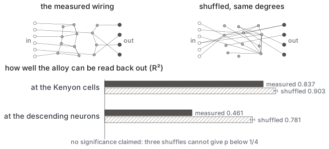
A degree-preserving shuffle carries composition better than the measured wiring. 300 compositions, cross-validated ridge decode of the eight element fractions:

No significance is quoted, and an earlier draft of this entry was wrong to quote one. Dividing the gap by the standard deviation of three shuffled graphs gives a standardised difference, not a tail probability: three null draws bound a one-sided randomisation test at p >= 1/4 however many compositions are decoded, because compositions and folds do not make more independent graphs. The effect is large; its significance is not established, and establishing it needs more null graphs, not more data through the same ones.

Confirmed against a second, independently constructed control. A configuration model, pairing out-stubs with in-stubs at random, holds both degree sequences exactly and gives +0.814, +0.789, +0.792 - the same answer. Both shuffles preserve the heavy tail the measured graph carries: its largest broadcaster has 7,570 outputs against a mean of 37.5, and the controls reach 6,970 and 6,952, so the gap is not the loss of hubs.

The measured wiring is not better than chance at delivering the composition to the motor output; it is substantially worse, and this survives the stronger control.

The metric is the wrong one, and that is a fault in the test rather than a defence of the result. A direct wire from the receptors to the descending neurons would score 1.0 and compute nothing; a random projection is near-lossless by construction. Recovering the input is close to the opposite of what a brain is for. What this measurement does establish is that no claim may rest on the connectome preserving information better than a random graph of the same shape, because it does not. Whether the wiring earns its place is decided end-to-end - the same forager, objective and budget, driven by the measured brain against the shuffled one - and until that is run, it is open.